Challenge

Week 4.1 - Genetic Algorithm

SSampreet Sabarad13 Apr 2022

Genetic Algorithm:

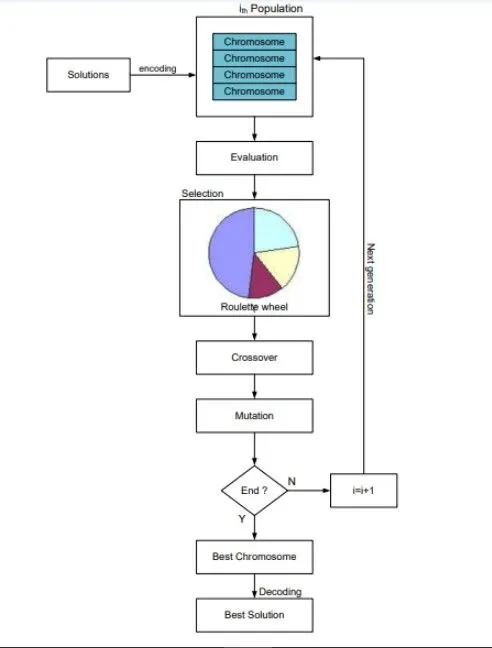
Genetic algorithm is a technique used to optimization and solve nonlinear/non differenciable optization problems.As Mr.Charles Darwin proposed the natural selection theory and evolution theory in the field of biology as it selects the best fit species,similar to that in matlab genetic algorithm it is used to find global minima in the optimization problem.GA begins with inital generation of candidate solutions that are validated with respect to objective function,if the optimum is found the result is showed else it undergoes with subsequent generation which includes selection,crossover & mutation.After the process it loops back to optimal calculation as process occurs as described further.

Graph of process occurance:

STEP-WISE EXPLAINATION OF THE CODE:

1.Use of commands, 'clear all','close all','clc' to erase all the previously programmed on workspace,graphs and command window.

2.As per problem statement we will begin to find the global maximum by optimization through genetic algorithm.

3.Defining the search space using linspace command

4.Meshing is done to have a matrix xx&yy.Also num_case is set to 50.

5.Inputs are given to function to to find f through 'for' loop.

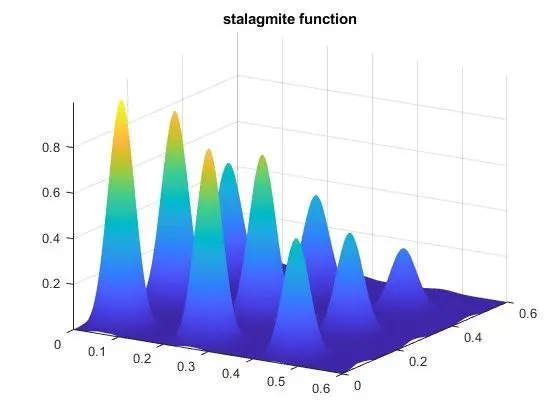
6.Surface is plotted using the plot command.

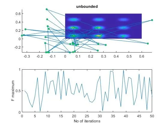
7.In the first case study is done for unbounded,Here genetic algorithm is used to find the x,y &f optimum values with 50 iterations using the 'for' loop.

8.tic and toc command is used calculate the times taken to calculate the process time.

9.Plotting is done against the xotp,yopt,fopt using 'surf' command and subplots are drawn in the same graph for Function maximum and numberof iterations.

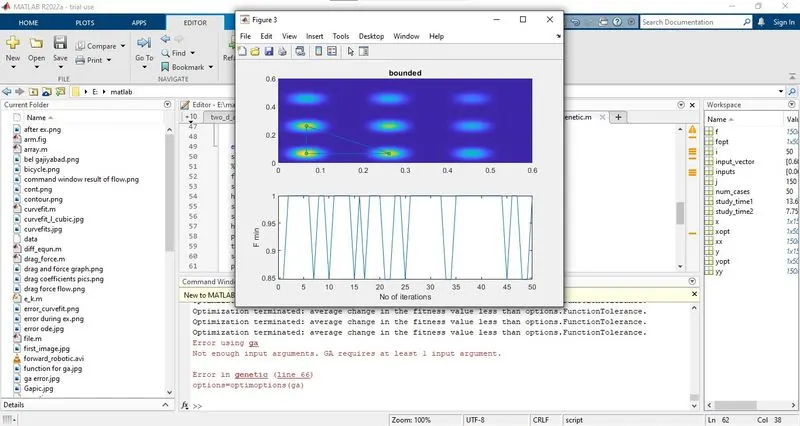
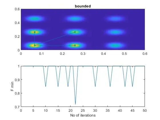
10.In the second case study is done by usng Boundry conditions,Here genetic algorithm is used to find the x,y &f optimum values by using the upper and lower boundry conditions with 50 iterations using the 'for' loop.

11.Plotting is done against the xotp,yopt,fopt using 'surf' command and subplots are drawn in the same graph for Function maximum and numberof iterations.

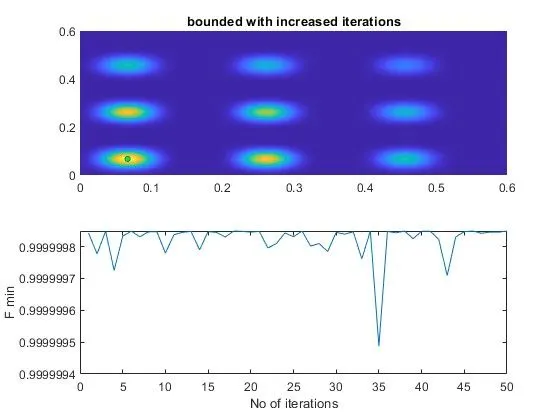
12.In the 3 case study is done to find the accurate result by increasing the population,Here genetic algorithm is used to find the x,y &f optimum values by using the upper and lower boundry conditions with 50 iterations using the 'for' loop.

13.Plotting is done against the xotp,yopt,fopt using 'surf' command and subplots are drawn in the same graph for Function maximum and numberof iterations.

MAIN CODE:

clear all
close all
clc
%Program to calculate global maxima 
%defining search space
x=linspace(0,0.6,150);
y=linspace(0,0.6,150);
%meshing
[xx,yy]=meshgrid(x,y)
num_cases=50;
for i=1:length(xx);
for j=1:length(yy);
    input_vector(1)=xx(i,j);
    input_vector(2)=yy(i,j);
  f(i,j)=stalagmite(input_vector)  ;
end
end
surfc(xx,yy,-f)
shading interp
title('stalagmite function')
%STUDY CASE 1 -Unbounded
tic
for i=1:num_cases
    [inputs,fopt(i)]=ga(@stalagmite,2);
    xopt(i)=inputs(1);
    yopt(i)=inputs(2);
end
study_time1=toc;
%plotting
figure(2)
subplot(2,1,1)
hold on
surfc(x,y,-f)
shading interp
hold on
plot3(xopt,yopt,-fopt,'marker','o','markerSize',4,'markerfacecolor','g')
title('unbounded')
subplot(2,1,2)
plot(-fopt)
ylabel('F maximum')           %labeling
xlabel('No of iterations')
%STUDY CASE 2-BOUNDED
%Introducing the boundry conditions for ga
tic;
for i=1:num_cases
    [inputs,fopt(i)]=ga(@stalagmite,2,[],[],[],[],[0;0],[0.4;0.4]);
    xopt(i)=inputs(1);
    yopt(i)=inputs(2);
end
study_time2=toc;
%plotting
figure(3)
subplot(2,1,1)
hold on
surfc(x,y,-f)
shading interp
hold on
plot3(xopt,yopt,-fopt,'marker','o','markerSize',4,'markerfacecolor','g')
title('bounded')
subplot(2,1,2)
plot(-fopt)
ylabel('F min')             %LABELING
xlabel('No of iterations')
%STUDY CASE3-BOUNDED WITH INCREASING THE POPULATION
%increased iterations
options=optimoptions('ga')
options=optimoptions(options,'populationsize',200)
for i=1:num_cases
    [inputs,fopt(i)]=ga(@stalagmite,2,[],[],[],[],[0;0],[0.4;0.4],[],[],options);
    xopt(i)=inputs(1);
    yopt(i)=inputs(2);
end
study_time3=toc;
%plotting
figure(4)
subplot(2,1,1)
hold on
surfc(x,y,-f)
shading interp
hold on
plot3(xopt,yopt,-fopt,'marker','o','markerSize',4,'markerfacecolor','g')
title('bounded with increased iterations')
subplot(2,1,2)
plot(-fopt)
ylabel('F min')            %LABELING
xlabel('No of iterations')

Function explaination:

1.Define the stalagmite function and assign the input variables

2.Define the function as per given formula as shown below:

f1=(sin(5.1*pi*x+(0.5)))^6 ;

f2=(sin(5.1*pi*y+(0.5)))^6 ;

f3=exp(-4*log(2)*(((x-0.0667)^2)/0.64));

f4=exp(-4*log(2)*(((y-0.0667)^2)/0.64));

3.While defining the final equation use '-' sign to find the global maxima.

Function CODE:

function [f]=stalagmite(input_vector)
x=input_vector(1);
y=input_vector(2);
f1=(sin(5.1*pi*x+(0.5)))^6 ;
f2=(sin(5.1*pi*y+(0.5)))^6 ;
f3=exp(-4*log(2)*(((x-0.0667)^2)/0.64));
f4=exp(-4*log(2)*(((y-0.0667)^2)/0.64));
f=-(f1*f2*f3*f4);
end

2.Errors occured during the excution:

Error occured due to missing the ' ' (apostropy) sign it was later rectified by appling it.

Error image