Challenge

Project 2 - Rankine cycle Simulator

SSampreet Sabarad18 Apr 2022

Rankine cycle Simulator:

'The Rankine cycle is an idealized thermodynamic cycle describing the process by which certain heat engines, such as steam turbines or reciprocating steam engines, allow mechanical work to be extracted from a fluid as it moves between a heat source and heat sink'.

Description of the process:

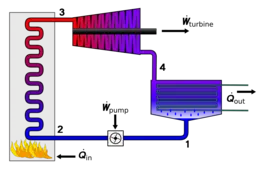
Process 1–2: The working fluid is pumped from low to high pressure. As the fluid is a liquid at this stage, the pump requires little input energy. Process 1-2 is isentropic compression.
Process 2–3: The high-pressure liquid enters a boiler, where it is heated at constant pressure by an external heat source to become a dry saturated vapour. The input energy required can be easily calculated graphically, using an enthalpy–entropy chart (h–s chart, or Mollier diagram), or numerically, using steam tables or software. Process 2-3 is constant pressure heat addition in boiler.
Process 3–4: The dry saturated vapour expands through a turbine, generating power. This decreases the temperature and pressure of the vapour, and some condensation may occur. The output in this process can be easily calculated using the chart or tables noted above. Process 3-4 is isentropic expansion.
Process 4–1: The wet vapour then enters a condenser, where it is condensed at a constant pressure to become a saturated liquid. Process 4-1 is constant pressure heat rejection in condenser.

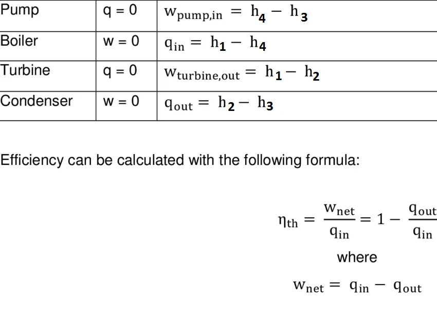
Equations used :

Specific steam consumption (SSC): It is the amount of steam required to produce unit work.

1.Step-wise explanation of your code.

Use of the command 'close all' ,'clear all','clc' to erase all the previously programmed graphs,workspace & command Window/
Inputs are assigned using 'input' command to enter the inetial values as turbine pressure input,output and input temperature.
Extracting the data for each perticular state using from XStream table.
Each state points has properties like Temperature,pressure,enthalpy,entropy,specific heat at constant presssure & at constant volume.
For each state points property values are extracted using 'XStream' and in the bracket we should specify the required data as per XStream rule and mention the perticular property value at which you need the data.
Using each property data at state points the outputs like work done by turbine/pump,heat supplied/rejected,specfic steam consumption,efficiency are calculated by the rankine cycle relations.
calculation of temp,entropy,enthalpy at vapour and liquid phase.
The curve is drwan using 'linspace' for the points in liquid & vapour region.
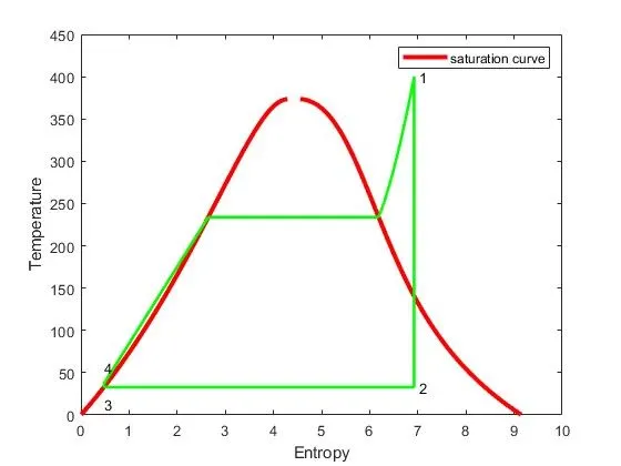
Also,using linspace command we are calculating temp v/s entropy points for a region at vapour state & points from (s6,t6) to (s1,t1) as it a curve.
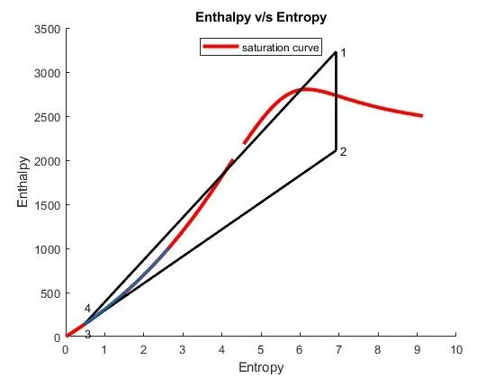
Plotting is done using 'plot' command for the T-s graph and H-S graph
During plotting of the H-s graph as we complete points from (s1,t1),to(s2,t2),to (s3,t3) to (s4,t4) we need to connect the line from s4 to s1 using linspace command as it is a curve including points 5 & 6 respectively.
Later,labeling is done by 'xlabel' & 'ylabel' and numbering is done using 'text' command.
Legend command is used for mention of the curve in the graph
Final required outputs with state points are displayed using 'fprintf' command, which appears in command window.

CODE FOR THE PROGRAM:

close all
clear all
clc
disp('RANKINE CYCLE')
disp('1-2 Isentropic expansion of turbine')
disp('2-3 Isothermal heat rejection from condenser')
disp('3-4 Isentropic compression through pump ')
disp('4-1 Isothermal heat addition')
%Inputs
p1=input('pressure at inlet of turbine(in bar):  ')
t1=input('Temperature at inlet of turbine(in degree C):  ')
p2=input('pressure at outlet of turbine(in bar):  ')

%Extracting data
h1=XSteam('h_pt',p1,t1);
s1=XSteam('s_pt',p1,t1);

%state 2
s2=s1;
sf2=XSteam('sL_p',p2);
sg2=XSteam('sV_p',p2);
x2=(s2-sf2)/(sg2-sf2);
hf2=XSteam('hL_p',p2);
hg2=XSteam('hV_p',p2);
h2=hf2+(x2*(hg2-hf2));

%state3
p3=p2;
s3=XSteam('sL_p',p3);
h3=XSteam('hL_p',p3);

%state4
s4=s3;
p4=p1;

%work done by turbine
wt=h1-h2;

%heat reject
Qout=h2-h3;

%pump work
v3=XSteam('vL_p',p2);
wp=v3*(p4-p3)*100;
h4=wp+h3;

%heat addition
Qin=h1-h4;

%net work
Wnet=wt-wp;
%Thermal efficiency
EFC=(Wnet/Qin)*100;

%specific steam consumption
ssc=(3600/Wnet);

%calculating saturation temperatures
t3=XSteam('Tsat_p',p3);
t2=t3;
cp4=XSteam('Cp_ps',p4,s4);
cv4=XSteam('Cv_ps',p4,s4);
gamma=cp4/cv4;
t4=t3/(p3/p4)^((gamma-1)/gamma);

%calculating temp,entropy,enthalpy at vapour and liquid phase
t6=XSteam('Tsat_p',p1);
s5=XSteam('sL_p',p1);
s6=XSteam('sV_p',p1);
h5=XSteam('hL_p',p1);
h6=XSteam('hV_p',p1);
t5=t6;

%plotting curve
Z=linspace(0,400,1000);
for i=1:length(Z)
    sf(i)=XSteam('sL_T',Z(i));
    sg(i)=XSteam('sV_T',Z(i));
    hf(i)=XSteam('hL_T',Z(i));
    hg(i)=XSteam('hV_T',Z(i));
end
%plotting T-s dia
figure(1)
plot(sf,Z,'Color','r','LineWidth',3)
hold on
plot(sg,Z,'Color','r','LineWidth',3)
hold on
plot([s1 s2],[t1 t2],'Color','g','LineWidth',2)
hold on
plot([s2 s3],[t2 t3],'Color','g','LineWidth',2)
hold on
plot([s3 s4],[t3 t4],'Color','g','LineWidth',2)
hold on
plot([s4 s5],[t4 t5],'Color','g','LineWidth',2)
hold on
plot([s5 s6],[t5 t6],'Color','g','LineWidth',2)
hold on

%line from (s6,t6) to (s1,t1)
ss=linspace(s6,s1,1000);
for j=1:length(ss);
    Tc1(j)=XSteam('T_ps',p1,ss(j));
end

plot(ss,Tc1,'g','LineWidth',2)
text(s1+0.1,t1,'1')
text(s2+0.1,t2,'2')
text(s3,t3-20,'3')
text(s4,t4+20,'4')
xlabel('Entropy')
ylabel('Temperature')
legend('saturation curve')

%plotting H-s
figure(2)
hold on
plot(sf,hf,'LineWidth',3,'Color','r')
plot(sg,hg,'LineWidth',3,'Color','r')
plot([s1 s2],[h1 h2],'LineWidth',2,'Color','k')
plot([s2 s3],[h2 h3],'LineWidth',2,'Color','k')
plot([s3 s4],[h3 h4],'LineWidth',2,'Color','k')

hc=linspace(h4,h5,100);
for k=1:length(hc)
    sch(k)=XSteam('s_ph',p1,hc(k));
end
plot(sch,hc,'LineWidth',2)
plot([s4 s1],[h4 h1],'LineWidth',2,'Color','k')
for o=1:length(ss)
    hc1(o)=XSteam('h_ps',p1,ss(o));
end
plot(sch,hc,'LineWidth',2)
text(s1+0.1,h1,'1')
text(s1+0.1,h2,'2')
text(s3,h3-100,'3')
text(s4,h4+200,'4')
title('Enthalpy v/s Entropy')
xlabel('Entropy')
ylabel('Enthalpy')
legend('saturation curve','location','north')

%Results
fprintf('RESULTS\n')
%state point 1
fprintf('STATE POINT 1:\n');
fprintf('Pressure at p1:  %9.5f bar \n',p1);
fprintf('Temperature at t1:%9.5f c \n',t1);
fprintf('Enthalpy at h1:%9.5f kj/kg \n',h1);
fprintf('Entropy at s1:%9.5f kj/kgk \n',s1);
%state point 2
fprintf('STATE POINT 2: \n');
fprintf('Pressure at p2:%9.5f bar \n',p2);
fprintf('Temperature at t2:%9.5f c \n',t2);
fprintf('Enthalpy at h2:%9.5f kj/kg \n',h2);
fprintf('Entropy at s2:%9.5f kj/kgk \n',s2);
%state point 3
fprintf('STATE POINT 3:\n');
fprintf('Pressure at p3:%9.5f bar \n',p3);
fprintf('Temperature at t3:%9.5f c \n',t3);
fprintf('Enthalpy at h3:%9.5f kj/kg \n',h3);
fprintf('Entropy at s3:%9.5f kj/kgk \n',s3);
%state point 4
fprintf('STATE POINT 4:\n');
fprintf('Pressure at p4:%9.5f bar \n',p4);
fprintf('Temperature at t4:%9.5f c \n',t4);
fprintf('Enthalpy at h4:%9.5f kj/kg\n ',h4);
fprintf('Entropy at s4:%9.5f kj/kgk \n',t4);
% Final Outputs
fprintf('Turbine work: %9.5f kj/kg \n',wt);
fprintf('pump work : %9.5f kj/kg \n',wp);
fprintf('Wnet: %9.5f total work in kj/kg \n',Wnet);
fprintf('Efficiency %9.5f \n',EFC);
fprintf('SSC(Specific Steam Consumption):%9.5f kj/kwh',ssc);

2.Errors faced while programming.

"There were no errors during programming but, there was a doubt in ploting the curves in T-s & H-s graphs which were resolved by having a one-on one section with support engineer."

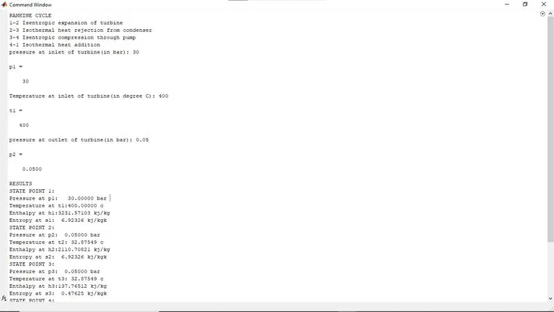
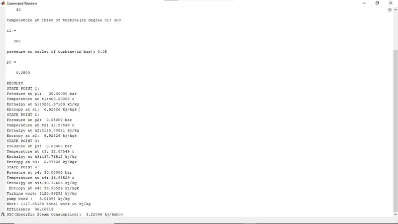
3.Final Outputs of command window:

Graph of Temperature v/s Entropy:

Graph of Enthalpy v/s Entropy:

Reference:

Project 2 - Rankine cycle Simulator

Ship work like this
in your own course.

Talk to a career counsellor

Ship work like thisin your own course.

Talk to a career counsellor

Ship work like this
in your own course.