Week 4.1 - Genetic Algorithm

Objective:

To write a code in MATLAB to optimise the stalagmite function and find the global maxima of the function.

Theory:

The genetic algorithm is a method for solving both constrained and unconstrained optimization problems that is based on natural selection, the process that drives biological evolution. The genetic algorithm repeatedly modifies a population of individual solutions. At each step, the genetic algorithm selects individuals from the current population to be parents and uses them to produce the children for the next generation. Over successive generations, the population "evolves" toward an optimal solution. You can apply the genetic algorithm to solve a variety of optimization problems that are not well suited for standard optimization algorithms, including problems in which the objective function is discontinuous, nondifferentiable, stochastic, or highly nonlinear. The genetic algorithm can address problems of mixed integer programming, where some components are restricted to be integer-valued.

The genetic algorithm uses three main types of rules at each step to create the next generation from the current population:

• Selection rules select the individuals, called parents, that contribute to the population at the next generation. The selection is generally stochastic, and can depend on the individuals' scores.
• Crossover rules combine two parents to form children for the next generation.
• Mutation rules apply random changes to individual parents to form children.

Difference between classical algorithm and genetic algorithm:

Classical algorithm:

• Generates a single point at each iteration. The sequence of points approaches an optimal solution.
• Selects the next point in the sequence by a deterministic computation.
• Typically converges quickly to a local solution.

Genetic algorithm:

• Generates a population of points at each iteration. The best point in the population approaches an optimal solution.
• Selects the next population by computation which uses random number generators.
• Typically takes many function evaluations to converge. May or may not converge to a local or global minimum.

ga Syntax:

x = ga(fun,nvars)

x = ga(fun,nvars,A,b)

x = ga(fun,nvars,A,b,Aeq,beq)

x = ga(fun,nvars,A,b,Aeq,beq,lb,ub)

x = ga(fun,nvars,A,b,Aeq,beq,lb,ub,nonlcon)

x = ga(fun,nvars,A,b,Aeq,beq,lb,ub,nonlcon,options)

x = ga(fun,nvars,A,b,Aeq,beq,lb,ub,nonlcon,intcon)

x = ga(fun,nvars,A,b,Aeq,beq,lb,ub,nonlcon,intcon,options)

x = ga(problem)

[x,fval] = ga(___)

[x,fval,exitflag,output] = ga(___)

[x,fval,exitflag,output,population,scores] = ga(___)

where,

nvars - number of design variables.

Aeq - Aeq matrix for linear equality constraints.

beq - beq matrix for linear equality constraints.

lb - lower bound for x.

ub - upper bound for x.

nonlcon - non linear constraint function.

options - options created by optimoptions.

x = ga(fun,nvars) finds a local unconstrained minimum, x, to the objective function, fun. nvars is the dimension (number of design variables) of fun.

x = ga(fun,nvars,A,b) finds a local minimum x to fun, subject to the linear inequalities A*x ≤ b. ga evaluates the matrix product A*x as if x is transposed (A*x').

x = ga(fun,nvars,A,b,Aeq,beq) finds a local minimum x to fun, subject to the linear equalities Aeq*x = beq and A*x ≤ b. (Set A=[] and b=[] if no linear inequalities exist.) ga evaluates the matrix product Aeq*x as if x is transposed (Aeq*x').

x = ga(fun,nvars,A,b,Aeq,beq,lb,ub) defines a set of lower and upper bounds on the design variables, x, so that a solution is found in the range lb ≤ x ≤ ub. (Set Aeq=[] and beq=[] if no linear equalities exist.)

x = ga(fun,nvars,A,b,Aeq,beq,lb,ub,nonlcon) subjects the minimization to the constraints defined in nonlcon. The function nonlcon accepts x and returns vectors C and Ceq, representing the nonlinear inequalities and equalities respectively. ga minimizes the fun such that C(x) ≤ 0 and Ceq(x) = 0. (Set lb=[] and ub=[] if no bounds exist.)

x = ga(fun,nvars,A,b,Aeq,beq,lb,ub,nonlcon,options) minimizes with the default optimization parameters replaced by values in options. (Set nonlcon=[] if no nonlinear constraints exist.) Create options using optimoptions.

x = ga(fun,nvars,A,b,Aeq,beq,lb,ub,nonlcon,intcon) or x = ga(fun,nvars,A,b,Aeq,beq,lb,ub,nonlcon,intcon,options) minimizes with the default optimization parameters replaced by values in options. (Set nonlcon=[] if no nonlinear constraints exist.)

x = ga(problem) finds the minimum for problem, a structure described in problem.

[x,fval] = ga(___) for any previous input arguments, also returns fval, the value of the fitness function at x.

[x,fval,exitflag,output] = ga(___) an integer identifying the reason the algorithm terminated, and output, a structure that contains output from each generation and other information about the performance of the algorithm.

[x,fval,exitflag,output,population,scores] = ga(___) returns a matrix population, whose rows are the final population, and a vector scores, the scores of the final population.

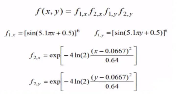
Stalagmite function:

MATLAB Program:

Function program:

function [f] = stalagmite(input_vector)

x = input_vector(1);
y = input_vector(2);

f1x = (sin(5.1*pi*x+0.5))^6;
f1y = (sin(5.1*pi*y+0.5))^6;

f2x = exp((-4*log(2)*(x-0.0667)^2)/0.64);
f2y = exp((-4*log(2)*(y-0.0667)^2)/0.64);

f = -(f1x*f2x*f1y*f2y);

end

Main program:

clear all
close all
clc

% Defining our search space
x = linspace(0,0.6,150);
y = linspace(0,0.6,150);
num_cases = 50;

% Creating two dimensional mesh
[xx yy] = meshgrid(x,y);


for i = 1:length(xx)
    for j = 1:length(yy)
        input_vector(1)=xx(i,j);
        input_vector(2)=yy(i,j);
        f(i,j)=stalagmite(input_vector);
    end
end

tic
% Study 1 - Statistical behaviour
for i=1:num_cases
    [inputs,fopt(i)]=ga(@stalagmite,2);
    xopt(i)= inputs(1);
    yopt(i)= inputs(2);
end
study1_time = toc;

figure(1)
subplot(2,1,1)
hold on
surfc(x,y,-f)
shading interp
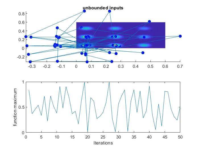
plot3(xopt,yopt,-fopt,'marker','o','markerfacecolor','b')
title('unbounded inputs')
subplot(2,1,2)
plot(-fopt)
xlabel('Iterations')
ylabel('function maximum')

tic
% Study 2- Statistical behaviour with lower and upper bounds
for i=1:num_cases
    [inputs,fopt1(i)] = ga(@stalagmite,2,[],[],[],[],[0,0],[0.6,0.6]);
    xopt1(i) = inputs(1);
    yopt1(i) = inputs(2);
end
study2_time = toc;

figure(2)
subplot(2,1,1)
hold on
surfc(x,y,-f)
shading interp
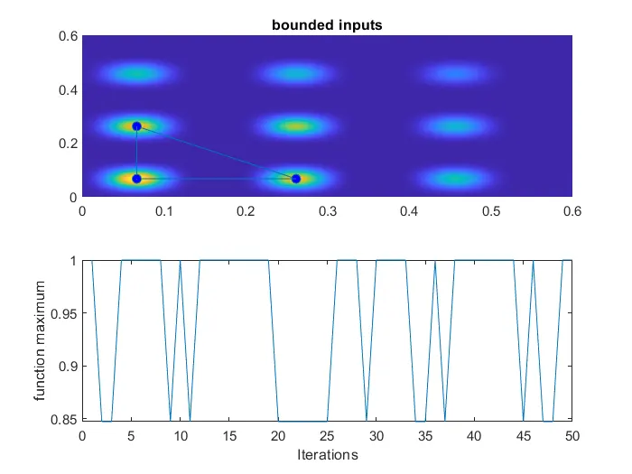
plot3(xopt1,yopt1,-fopt1,'marker','o','markerfacecolor','b')
title('bounded inputs')
subplot(2,1,2)
plot(-fopt1)
xlabel('Iterations')
ylabel('function maximum')


%Study 3- Increasing population size
options = optimoptions('ga')
options = optimoptions(options,'PopulationSize',250)

for i=1:num_cases
    [inputs,fopt2(i)] = ga(@stalagmite,2,[],[],[],[],[0,0],[0.6,0.6],[],[],options);
    xopt2(i) = inputs(1);
    yopt2(i) = inputs(2);
end
study3_time = toc;

figure(3)
subplot(2,1,1)
hold on
surfc(x,y,-f)
shading interp
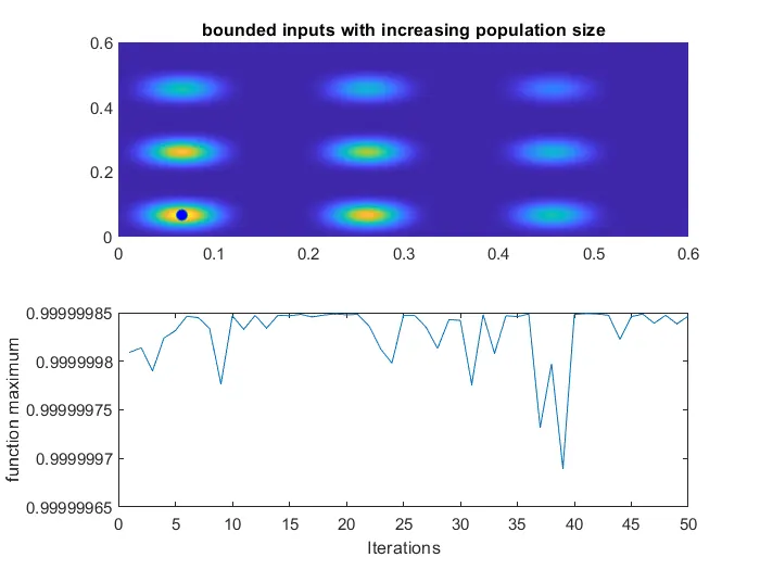
plot3(xopt2,yopt2,-fopt2,'marker','o','markerfacecolor','b')
title('bounded inputs with increasing population size')
subplot(2,1,2)
plot(-fopt2)
xlabel('Iterations')
ylabel('function maximum')

Explanation:

clear all - This MATLAB function removes all variables from the current workspace, releasing them from system memory.

close all - This MATLAB function closes the current figure.

clc - This MATLAB function clears all the text from the Command Window, resulting in a clear screen.

linspace - This MATLAB function returns a row vector of 100 evenly spaced points between x1 and x2.

meshgrid - This MATLAB function returns 2-D grid coordinates based on the coordinates contained in vectors x and y.

ga - This MATLAB function finds a local unconstrained minimum, x, to the objective function, fun.

tic - This MATLAB function works with the toc function to measure elapsed time.

toc - This MATLAB function reads the elapsed time since the stopwatch timer started by the call to the tic function.

subplot - This MATLAB function divides the current figure into an m-by-n grid and creates axes in the position specified by p.

surfc - This MATLAB function creates a three-dimensional surface plot with a contour plot underneath.

shading - This MATLAB function each mesh line segment and face has a constant color determined by the color value at the endpoint of the segment or the corner of the face that has the smallest index or indices.

plot3 - This MATLAB function plots coordinates in 3-D space.

title - This MATLAB function adds the specified title to the current axes or standalone visualization.

xlabel - This MATLAB function labels the x-axis of the current axes or standalone visualization.

ylabel - This MATLAB function labels the y-axis of the current axes or standalone visualization.

plot - This MATLAB function creates a 2-D line plot of the data in Y versus the corresponding values in X.

hold on - This MATLAB function retains plots in the current axes so that new plots added to the axes do not delete existing plots.

Results:

The graphs for all 3 studies and for F maximum vs no. of iterations are given below.