Week 4.1 - Genetic Algorithm

Aim:

The main aim of this challenge is to write a code in MATLAB to optimise the stalagmite function and find the global maxima of the function.

Concept of Genetic Algorithm:

*Genetic Algorithms are a family of computational models inspired by evolution. These algorithms encode a potential solution to a specific problem on a simple chromosome-like data structure and apply recombination operators to these structures as as to preserve critical information. Genetic algorithms are often viewed as function optimizer, although the range of problems to which genetic algorithms have been applied are quite broad.

*An implementation of genetic algorithm begins with a population of (typically random) chromosomes. One then evaluates these structures and allocated reproductive opportunities in such a way that these chromosomes which represent a better solution to the target problem are given more chances to `reproduce’ than those chromosomes which are poorer solutions. The ‘goodness’ of a solution is typically defined with respect to the current population.

How GENETIC ALGORITHM works:

Genetic Algorithm works by the process of natural selection. It starts from an initial, maybe random population which represent a pool of all possible solutions to a problem. Then these population undergoes several processed such as Selection, Cross-Over and Mutation and finally produces the best results 0ptimal solution at the end of the process.

SYNTAX FOR GA:

1. x = ga(fun,nvars) finds a local unconstrained minimum, x,

where,

fun = objective function

nvars = number of design variables

2. x = ga(fun,nvars,A,b,Aeq,beq,lb,ub) defines a set of lower and upper bounds on the design variables, x, so that a solution is found in the range.

where,

fun = objective function

nvars = number of design variables

lb = lowerbounds

ub = upperbounds

3. x= ga(fun,nvars,A,b,Aeq,beq,lb,ub,nonlcon,intcon,options) minimizes with the default optimization parameters replaced by values in options. Create options using optimoptions.

where,

fun = objective function

nvars = number of design variables

lb = lowerbounds

ub = upperbounds

nonlcon = nonlinear constraints

intcon = positive integer vectors

options = optimisation options / optimoptions

Main code: To find global maxima of the function.

clear all
close all 
clc

x=linspace(0,0.6,150);
y=linspace(0,0.6,150);
num_cases=50;
[xx yy]=meshgrid(x,y)

%evaluating
for i=1:length(xx)
    for j=1:length(yy)
        input_vector(1)=xx(i,j);
         input_vector(2)=yy(i,j);
        f(i,j)=stalagmite(input_vector);
    end
end


%study 1= statistical behavior
tic
for i=1:num_cases
    [inputs,fopt(i)]=ga(@stalagmite,2)
    xopt(i)=inputs(1)
    yopt(i)=inputs(2)
end

study_time1=toc
figure(1)
%plotting
subplot(2,1,1)
hold on
surfc(x,y,-f)
shading interp

plot3(xopt,yopt,-fopt,'marker','o','markersize',5,'markerfacecolor','r')
title('unbounded inputs')

subplot(2,1,2)
plot(-fopt)
xlabel('Iterations')
ylabel('Function maximum')

%study2=statistical behavior with upper and lower bounds
tic
for i=1:num_cases
    [inputs,fopt(i)]=ga(@stalagmite,2,[],[],[],[],[0;0],[0.6;0.6]);
    xopt(i)=inputs(1)
    yopt(i)=inputs(2)
end
study_2=toc

figure(2)
% plotting
subplot(2,1,1)
hold on
surfc(x,y,-f)
shading interp
plot3(xopt,yopt,-fopt,'marker','o','markersize',5,'markerfacecolor','r')
title('bounded inputs')
subplot(2,1,2)
plot(-fopt)
xlabel('Iterations')
ylabel('Function maximum')

%study3=Increasing the GA iterations

options=optimoptions('ga')
options=optimoptions(options,'populationsize',300);
tic
for i=1:num_cases
    [inputs,fopt(i)]=ga(@stalagmite,2,[],[],[],[],[0;0],[0.6;0.6],[],[],options);
    xopt(i)=inputs(1)
    yopt(i)=inputs(2)
end
study_time3= toc

figure(3)
%plotting
subplot(2,1,1)
hold on
surfc(x,y,-f)
shading interp
plot3(xopt,yopt,-fopt,'marker','o','markersize',5,'markerfacecolor','r')
title('Increasing Iterations of Generic Algorithm')

subplot(2,1,2)
plot(-fopt)
xlabel('Iterations')
ylabel('Function maximum')

Code Explaination:

1. clear all
close all
clc

these commands are used and then our code gets started.

2.The x and y inputs are take by using linspace command, and the meshgrid is created.

3.For loop is used for the evaluation purpose where the input vectors are given and then the stalagmite function gets called and the for loop gets ended.

Studytime 1 = Statistical behavior

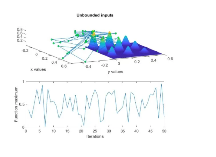
4. In the study time 1 for loop gets started withe the necessory xopt and yopt inputs and the loop get ended.Here the tic and toc commands are used to calculate the run time of the program.

5.The plotting is done by giving the necessory data like subplot, xlabel,ylabel,title. The code for plotting is mentioned below

%plotting
subplot(2,1,1)
hold on
surfc(x,y,-f)
shading interp

plot3(xopt,yopt,-fopt,'marker','o','markersize',5,'markerfacecolor','r')
title('unbounded inputs')

subplot(2,1,2)
plot(-fopt)
xlabel('Iterations')
ylabel('Function maximum')

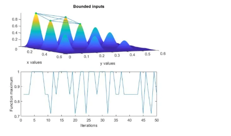
Studytime2 = Statistical behavior with upper and lower bounds.

7. Similar to the study time 1 the data is given and the for loop gets executed. Then the values are entered and the plotting is done. The code used for plotting is given below.

% plotting
subplot(2,1,1)
hold on
surfc(x,y,-f)
shading interp
plot3(xopt,yopt,-fopt,'marker','o','markersize',5,'markerfacecolor','r')
title('bounded inputs')
subplot(2,1,2)
plot(-fopt)
xlabel('Iterations')
ylabel('Function maximum')

8.Studytime3 = Increasing the Genetic Algorithm iterations.

options=optimoptions('ga')
options=optimoptions(options,'populationsize',300);

the code above indicates the increase in the population size.

And then the for loop gets executed with necessory inputs and the plotting gets done.

%plotting
subplot(2,1,1)
hold on
surfc(x,y,-f)
shading interp
plot3(xopt,yopt,-fopt,'marker','o','markersize',5,'markerfacecolor','r')
title('Increasing Iterations of Generic Algorithm')

subplot(2,1,2)
plot(-fopt)
xlabel('Iterations')
ylabel('Function maximum')

Code for stalagmite function:

function f=stalagmite(input_vector)
x=input_vector(1);
y=input_vector(2);
f1=(sin(5.1*pi*x+0.5))^6;
f2=(sin(5.1*pi*y+0.5))^6;
f3=exp((-4* log(2)*(x-0.0667)^2)/0.64);
f4=exp((-4*log(2)*(y-0.0667)^2)/0.64);
f=-(f1*f2*f3*f4);
end

Result:

study 1: Statistical behavior

Study2: Statistical behavior with upper and lower bounds.

Study 3: Increasing the Genetic Algorithm iterations.

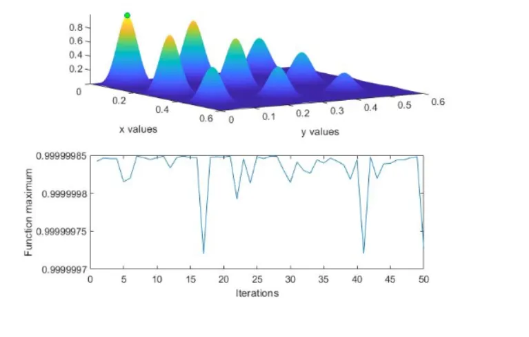
Thus the code is created with necessory plots showing the global maxima of the function.