Project 2 - Rankine cycle Simulator
Aim:
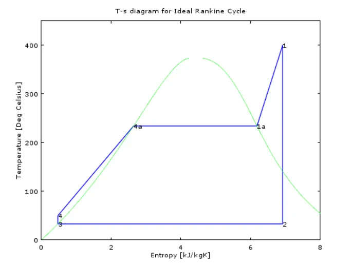
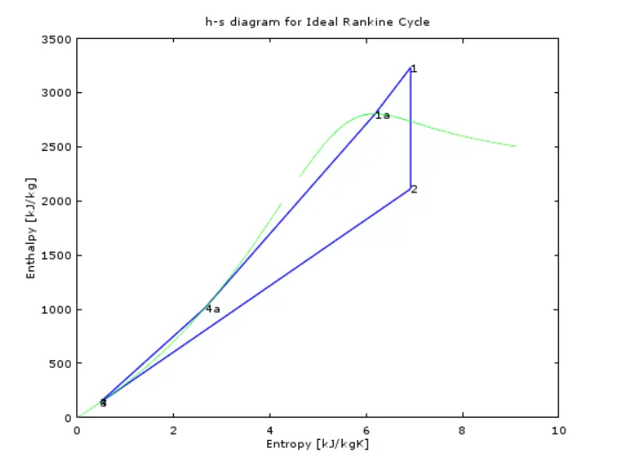
The main aim of this program is to write a code to calculate the state points of the Rankine Cycle based on user inputs and tp plot the required plots for T-s and h-s plots.
Rankine Cycle:
- The Rankine cycle is an idealized thermodynamic cycle describing the process by which certain heat engines, such as steam turbines or reciprocating steam engines, allow mechanical work to be extracted from a fluid as it moves between a heat source and heat sink.
Process1-2 -Isentropic Expansion
Process2-3- Constant Pressure Heat Rejection
Process3-4 -Isentropic Compression
Process4-1- Constant pressure Heat Addition
Process1-2 -Isentropic Expansion
An isentropic or adiabatic compression/expansion takes place when the compression/expansion of gas occurs with no heat energy flow in or out of the gas. Molecules do not interact and have no volume in an ideal gas. Pressure varies linearly with quantity.
Process2-3- Constant Pressure Heat Rejection
Constant Pressure Heat Rejection This process is the opposite of processes 2-3. In this process, the hot air from the turbine is again cooled and brought to its initial state so that it can be used again.
Process3-4 -Isentropic Compression
During a Rankine cycle, work is done on the fluid by the pumps between states 1 and 2 (isentropic compression). Work is done by the fluid in the turbine between stages 3 and 4 (isentropic expansion).
Process4-1- Constant pressure Heat Addition
Addition of heat at constant pressure to a gas results in Raising its temperature and doing external work When you heat a gas, both its vapor pressure and the volume it occupies increase. The individual gas particles become more energetic and the temperature of the gas increases.
Formula:
Net work output ,Wnet = Wt - Wp
Back work ratio,BW = (Wp/Wt)
Main code:
clear all
close all
clc

%process
fprintf('1-2 Isentropic Expansion')
fprintf('2-3 Constant Pressure Heat Rejection')
fprintf('3-4 Isentropic Compression')
fprintf('4-1 Constant pressure Heat Addition')

%initial Inputs to be entered in command window
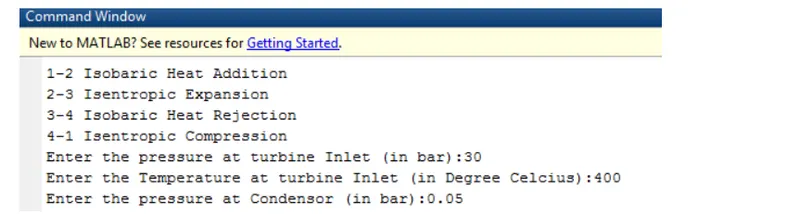
p1=input('Enter the turbine Inlet pressure (in bar):')
T1=input('Enter the turbine Inlet temperature (in Degree Celcius):')
p2=input('Enter the turbine Outlet pressure(in bar): ');

%State points calculation
%State point 1
h1 = XSteam('h_pt',p1,T1);
s1 = XSteam('s_pt',p1,T1)

%state point 2
s2=s1;
sf2 = XSteam('sL_p',p2);
sg2 = XSteam('sv_p',p2);
hf2 = XSteam('hl_p',P2)
hg2 = XSteam('hV_p',P2)
x2 = ((s2-sf2)/(sg2-sf))
h2 = hf2+ x2* (hg2-hf2);
T2 = XSteam('T_hs', h2,s2);

%State point 3
p3=p2;
s3 = XSteam('sl_p',p3);
h3 = XSteam('hl_p',p3);
T3 = T2;

%State point 4
s4 = s3;
P4 = p1;
Cp4= XSteam('Cp_ps',p4,s4)
Cv4 = XSteam('Cv_ps',p4,s4)
Y=Cp4/Cv4;
n=(Y-1)/Y;
T4 = T3*(p4/p3)^n;

%Work done by turbine
Wt = h1-h2;
%Work done to operate pump
V3 = XSteam('vL_P',p3);
h4 = h3 + Wp;
Wp = v3*(P4-p3)*100;
%Net Work
Wnet = Wt - Wp;

%Heat supplied
Qin = h1 - h4;
%Heat Rejected
Qout = h2 - h3;
%Thermal Efficiency
T_efficiency = (Wnet/Qin)*100;
%Specific steam Consumption
SSC = (3600/Wnet);
%Back Work ratio
BW = (Wp/Wt);
%Saurated Liquid and vapor points calculation
T6 = XSteam('Tsat_p',p1)
s5=XSteam('sl_p',p1)
s6=XSteam('sV_p',p1);
h5 = XSteam('hl_p',p1);
h6= XSteam('hV_p',p1);
T5 = T6;
%Printing results
fprintf('\n at state point 1 \n')
fprintf('p1=%f bar \n',p1)
fprintf('T1=%f Deg Celsius \n',T1)
fprintf('h1=%f kJ/kg \n',h1)
fprintf('s1=%f kJ/kgK \n',s1)

fprintf('\n at state point 2 \n')
fprintf('p2=%f bar \n',p2)
fprintf('T2=%f Deg Celsius \n',T2)
fprintf('h2=%f kJ/kg \n', h2)
fprintf('s2=%f kJ/kgk \n',s2)

fprintf('\n at state point 3 \n')
fprintf('p3=%f bar \n',p3)
fprintf('T3=%f Deg Celsius \n',T3)
fprintf('h3=%f kJ/kg \n',h3)
fprintf('s3=%f kJ/kgk \n',s3)

fprintf('\n at state point 4 \n')
fprintf('p4=%f bar \n',p4)
fprintf('T4=%f Deg Celsius \n',T4)
fprintf('h4=%f kJ/kg \n', h4)
fprintf('s4=%f kJ/kgk \n', s4)

fprintf('\n Work done by turbine = %f kJ/kg \n',wt)
fprintf('work done on pump=%f kJ/kg \n',wp)
fprintf('Net work done=%f kJ/kg \n',w_net)
fprintf('work ratio=%f \n',work_ratio)
fprintf('back work ratio=%f \n',back_work_ratio)
fprintf('Thermal efficiency=%f percent \n',cycle_efficiency)
%plotting Saturation curve and T-s diagram
T = linspace(1,374,400);
for i=1:length(T);
sf(i) = XSteam('sl_T',T (i));
sg(i)= XSteam('sV_T', T(i));
hf(i) = XSteam('hl_T',T(i));
hg(i)= XSteam('hv_T',T(i));
end

%plotting
figure(1)
hold on
plot(sf,T)
plot(sg,T)
plot([s1 s2],[T1 T2], [s2 s3],[T2 T3],[s3 s4],[T3 T4],[s4 s5],[T4 T5],[s5 s6],[T5 T6],[s6,s1],[T6,T1],'linewidth',1.5,'color','b')
text(s1+0.2,T1,'1')
text(s2+0.2,T2,'2')
text(s3+0.2, T3-4,'3')
text(s4-0.3, T4+4,'4')
text(s5-0,4, T5+5,'5')
text(s6+0.2, T6,'6')
xlabel('Entropy (kJ/kg)')
ylabel('Temperatur (KJ/kg)')
title('T-s diagram for Ideal Rankine Cycle')

% plotting
figure(2)
hold on
plot(sg, hg)
plot(sf, hf)
plot([s1 s2], [h1 h2],[s2 s3], [h2 h3], [s3 s4], [h3 h4],[s4 s1], [h4 h1],'linewidth',1.5,'color','g')
text(S1+0.1, h1,'1')
text(s2+0.1, h2,'2')
text(s3+0.2, h3-4, '3')
text(s4-0.3, h4+4, '4')
xlabel('Entropy (kJ/kg)')
ylabel('Enthalpy (kJ/K)' )
title('h-s diagram for Ideal Rankine Cycle')
Code Explaination:
1. The required input value are givenn in the process description.The initial inputs must be entered in the command window.
2.Then the state point values are given withthe required inputs.
%State point 1
h1 = XSteam('h_pt',p1,T1);
s1 = XSteam('s_pt',p1,T1)
%state point 2
s2=s1;
sf2 = XSteam('sL_p',p2);
sg2 = XSteam('sv_p',p2);
hf2 = XSteam('hl_p',P2)
hg2 = XSteam('hV_p',P2)
x2 = ((s2-sf2)/(sg2-sf))
h2 = hf2+ x2* (hg2-hf2);
T2 = XSteam('T_hs', h2,s2);
%State point 3
p3=p2;
s3 = XSteam('sl_p',p3);
h3 = XSteam('hl_p',p3);
T3 = T2;
%State point 4
s4 = s3;
P4 = p1;
Cp4= XSteam('Cp_ps',p4,s4)
Cv4 = XSteam('Cv_ps',p4,s4)
Y=Cp4/Cv4;
n=(Y-1)/Y;
T4 = T3*(p4/p3)^n;
3. Then the required formula is noted down in the editor
%Work done by turbine
Wt = h1-h2;
%Work done to operate pump
V3 = XSteam('vL_P',p3);
h4 = h3 + Wp;
Wp = v3*(P4-p3)*100;
%Net Work
Wnet = Wt - Wp;
%Heat supplied
Qin = h1 - h4;
%Heat Rejected
Qout = h2 - h3;
%Thermal Efficiency
T_efficiency = (Wnet/Qin)*100;
%Specific steam Consumption
SSC = (3600/Wnet);
%Back Work ratio
BW = (Wp/Wt);
4. Then the program to print the results are written
%Printing results
fprintf('\n at state point 1 \n')
fprintf('p1=%f bar \n',p1)
fprintf('T1=%f Deg Celsius \n',T1)
fprintf('h1=%f kJ/kg \n',h1)
fprintf('s1=%f kJ/kgK \n',s1)
fprintf('\n at state point 2 \n')
fprintf('p2=%f bar \n',p2)
fprintf('T2=%f Deg Celsius \n',T2)
fprintf('h2=%f kJ/kg \n', h2)
fprintf('s2=%f kJ/kgk \n',s2)
fprintf('\n at state point 3 \n')
fprintf('p3=%f bar \n',p3)
fprintf('T3=%f Deg Celsius \n',T3)
fprintf('h3=%f kJ/kg \n',h3)
fprintf('s3=%f kJ/kgk \n',s3)
fprintf('\n at state point 4 \n')
fprintf('p4=%f bar \n',p4)
fprintf('T4=%f Deg Celsius \n',T4)
fprintf('h4=%f kJ/kg \n', h4)
fprintf('s4=%f kJ/kgk \n', s4)
fprintf('\n Work done by turbine = %f kJ/kg \n',wt)
fprintf('work done on pump=%f kJ/kg \n',wp)
fprintf('Net work done=%f kJ/kg \n',w_net)
fprintf('work ratio=%f \n',work_ratio)
fprintf('back work ratio=%f \n',back_work_ratio)
fprintf('Thermal efficiency=%f percent \n',cycle_efficiency)
5.Then the linncpace command
T = linspace(1,374,400);
is used to generate the required values, and the for loop gets executed as the conditions are given.
6.Then the plotting is done with necessary inputs like xlabel,ylabel and title with the necessory plots.
Plots:
1. T-s diagram:
2. h-s diagram:
Result:
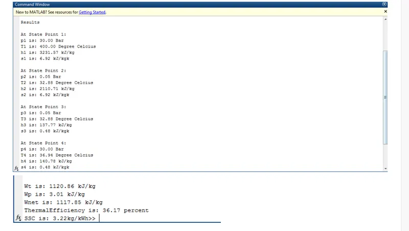
Thus the code for Rannkine Cycle Simulator is created with the necessary plot diagrams and code explaination