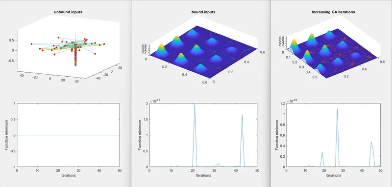
Week 4.1 - Genetic Algorithm

AIM

 To understand the concept of genetic algorithm and write the code to determine the global maxima.

OBJECTIVE

• To write a code in MATLAB to optimise the stalagmite function and find the global maxima of the function.
• To explain the concept of genetic algorithm and also explain the syntax ‘ga’ in MATLAB.
• To make a plot graphs for all 3 studies and for F maximum vs no of iterations. 

MAIN CODE

close

clear

clc

% Defining our search space

x = linspace(0,0.6,150);

y = linspace(0,0.6,150);

num_cases = 50;

[xx, yy] = meshgrid(x,y);

for k= 1:length(xx);

    for j = 1:length(yy);

        input_vector(1)=xx(k,j);

        input_vector(2)=yy(k,j);

        f(k,j) = stalagmite(input_vector);

    end

end

tic

%study 1 - satistical behaviour without bound limit

for i = 1:num_cases;

    [inputs,fopt(i)] = ga(@stalagmite,2);

     xopt(i) = inputs(1);

     yopt(i) = inputs(2);

end

study1_time = toc

figure (1)

subplot(2,1,1)

hold on

surfc (x, y,f)

shading interp

plot3(xopt,yopt,fopt,'marker','o','markersize',5, MarkerFaceColor='r')

title('unbound inputs')

subplot(2,1,2)

plot(fopt)

hold off

xlabel('Iterations')

ylabel('Function minimum')

%study 2 - statistical behaviour - with upper and lower bounds

tic

for i = 1:num_cases;

    [inputs,fopt(i)] = ga(@stalagmite,2,[],[],[],[],[0;0],[0.6;0.6]);

     xopt(i) = inputs(1);

     yopt(i) = inputs(2);

end

study2_time = toc

figure (2)

subplot(2,1,1)

hold on

surfc (x, y,f)

shading interp

plot3(xopt,yopt,fopt,'marker','o','markersize',5, MarkerFaceColor='r')

title('bound inputs')

subplot(2,1,2)

plot(fopt)

hold off

xlabel('Iterations')

ylabel('Function minimum')

%study 3 - Increasing GA iterations

options = optimoptions('ga');

options = optimoptions(options,'PopulationSize',200)

tic

for i = 1:num_cases;

    [inputs,fopt(i)] = ga(@stalagmite,2,[],[],[],[],[0;0],[0.6;0.6],[],[],options);

     xopt(i) = inputs(1);

     yopt(i) = inputs(2);

end

study3_time = toc

figure (3)

subplot(2,1,1)

hold on

surfc (x, y,f)

shading interp

plot3(xopt,yopt,fopt,'marker','o','markersize',5, MarkerFaceColor='r')

title('Increasing GA iterations')

subplot(2,1,2)

plot(fopt)

hold off

xlabel('Iterations')

ylabel('Function minimum')

FUNCTION CODE

function [f] = stalagmite (input_vector)

x = input_vector(1);

y = input_vector(2);

%formulas

f1x = (sin(5.1*pi*x+0.5)).^6;

f1y = (sin(5.1*pi*y+0.5)).^6;

f2x = exp(-4*log(2).*((x-0.0667).^2/0.64));

f2y = exp(-4*log(2).*((y-0.0667).^2/0.64));

f = -(f1x.*f2x.*f1y.*f2y);

end

EXPLANATION

• First of all we want to create a function by the given formula in the name of ‘stalagmite’. 
• In this function we make a small deference to determine the global maxima. Because the ‘ga’ find only minimum value so for that multiple the ‘-‘ in the last step of stalagmite function. 
• So we get all the data in the negative format so its is easy to find the global minima and we can remove the ‘-‘ and determine the global maxima. 
• For this code we are going make three separate studies that are unbound [statistical behaviour with out bound limits], bounded [statistical behaviour with upper and lower bound limits] and Increasing the iterations of Genetic algorithm.
• Then we giving the x and y values  by using ‘linspace’ command as ‘linspace(0,0.6,150)’. Here we are denoting that take 150 random data within the limit of 0 to 0.6.
• After that we are going to make two dimensional array by using the ‘meshgrid’ command. And denote that values are xx and yy.
• Then we are going run this genetic algorithm for fifty time for that we are going make new parameter named as ‘num_cases’ and give fifty as their value.
• We got all we want to make a study. So we open the for loop ‘k = 1:length(xx)’. Here we denoting the ‘k’  is equal to 1 to length of xx. So we get the k is equal to 150.
• We open the for loop ‘j= 1:length(xx)’. Here we denoting the ‘j’  is equal to 1 to length of yy. So we get the value for j is equal to 150.
• After that we are going to make the ‘f(k,j)’ by using the stalagmite function as ‘stalagmite(input_vector)’.
• Here we are not having the input values so we determine that as input_vector(1) = xx(k,j) and input_vector(2) = yy(k,j).
• After that we put end for both loop.
• Study 1 statistical behaviour open for loop ‘i = 1: num_cases’ here the value of num_cases is 50 here we are running the genetic algorithm for fifty values.
• After that we denote the array ‘[inputs, fopt(i)] = ga(@stalagmite,2)’.
• Here we open the ga command and denotes function and nvars (it is the dimension of this function).
• After that we are introduce the new variables they are xopt and yopt. Denote the xopt(i) is equal to input(1) and  yopt(i) is equal to input(2). 
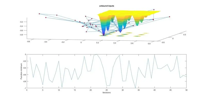
• Then we are going make a plot for this first study.
• To determine the time we add tic in the beginning of the for loop and add toc after the end of the for loop as study1_time.
• Figure (1) in this figure we are going to make two sub plot one with using the surfc command  to create the surface and using plot3 command we make a plot of optimum value of x,y,f using the marker command we make a maker in the size of 5.
• And in second sub plot we determine the change of the ‘fopt’.
• We gave the xlabel and ylabel as Iteration and Function minimum.
• Here the plot looks like this
•  
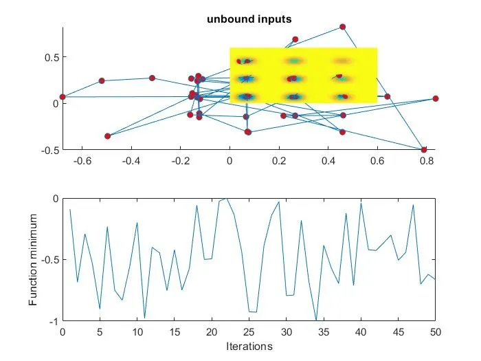
• In this first study we get 50 random data as num cases. The plot look messy and we get values that above the given data so we can’t able to determine the global maxima.
• So we go for study two by giving the bound limits.
• Here we give a bound limits as [0;0] and [0.6;0.6] in ga command.
• Because the given data for x and y are started with 0 and ended with 0.6.
• If we use the bound limit in ga command. We have to determine the A, b, Aeq and beq in the ga command.
• Here the A and b is a Linear inequality constraints and Aeq and beq are Linear equality constraints.
• We don’t give the values this syntax in the study two. 
• After this we going to make all the steps same as study 1.
• To determine the time we add tic in the beginning of the for loop and add toc after the end of the for loop as study2_time.
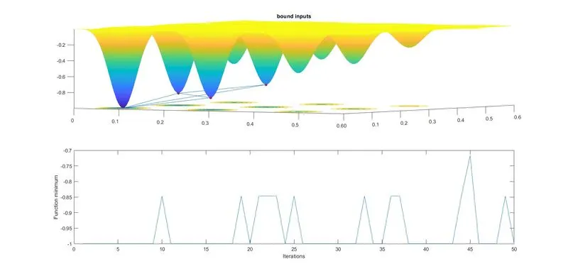
• Figure (2) in this figure we are going to make two sub plot one with using the surfc command  to create the surface and using plot3 command we make a plot of optimum value of x,y,f using the marker command we make a maker in the size of 5.
• And in second sub plot we determine the change of the ‘fopt’.
• We gave the xlabel and ylabel as Iteration and Function minimum.
• Here the plot looks like this
• 
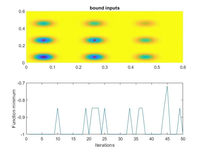
• This study is far better than the study one but in this study also we can’t able to determine the global maxima.
• So we are going to study three in this we are going to do ‘optimization’ 
• For that we use the command ‘options = optimoptions(‘ga’)’. Here we denote the solver name and the solver name in this code is ga  
• After this we are going to use the ‘options=optimoptions(options,’PopulationSize’,200)' and this command we denote the oldoption as options and we name this as ‘PopulationSize’ and value as 200. 
• If we give values as 200 we get 200 value in between the 0 to 0.6.
• After the creation of the options we are going to use same steps followed the above study but we make a small deference here by using options in the ga command.
• In this study we give a bound limits as [0;0] and [0.6;0.6] in ga command and we add options in the end of the ga command.
• We have to determine the A, b, Aeq, beq, nonlcon and intcon in the ga command.
• Here the A and b is a Linear inequality constraints and Aeq and beq are Linear equality constraints. Nonlcon is a non linear constraint. Intcon is integer constraint.
• We don’t give the values this syntax in the study three.
• After this we going to make all the steps same as study 1.
• To determine the time we add tic in the beginning of the for loop and add toc after the end of the for loop as study3_time.
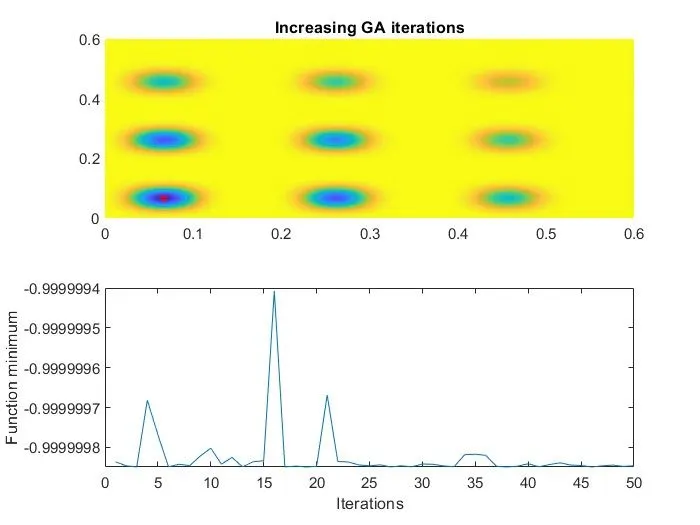
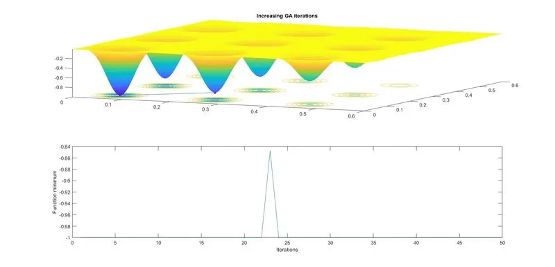
• Figure (3) in this figure we are going to make two sub plot one with using the surfc command  to create the surface and using plot3 command we make a plot of optimum value of x,y,f using the marker command we make a maker in the size of 5.
• And in second sub plot we determine the change of the ‘fopt’.
• We gave the xlabel and ylabel as Iteration and Function minimum.
• Here the plot looks like this
• 

OUTPUT

FOR STUDY 1 - SATISTICAL BEHAVIOUR WITHOUT BOUND LIMIT

FOR STUDY 2 - WITH BOUND LIMIT

FOR STUDY 3 - INCREASING GA ITERATIONS

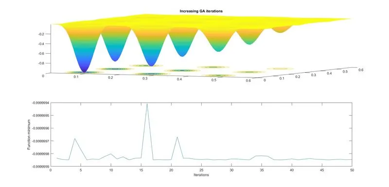
From the above three studies we can able to determine the global maxima by the study 3 we conclued that the global maxima of give data is 0.99999975.   

EXPLANATION

GENETIC ALGORITHM

 The Genetic algorithm is that run the data in optimisation technique based the principle we can to the system and it will give optimum solution or answer in it. 

This is syntax we used in this program x = ga(fun,nvars,A,b,Aeq,beq,lb,ub,nonlcon,intcon,options)

for the above ga syntax we have determine the data fun is a function so we use stalagmite unction in it. The nvars to determine the dimension of this function. Here the A and b is a Linear inequality constraints and Aeq and beq are Linear equality constraints. lb and ub is the lower bound and upper bound. Nonlcon is a non linear constraint. Intcon is integer constraint. options is optimization options we obtain by the command 'optimoptions'.

ERRORS

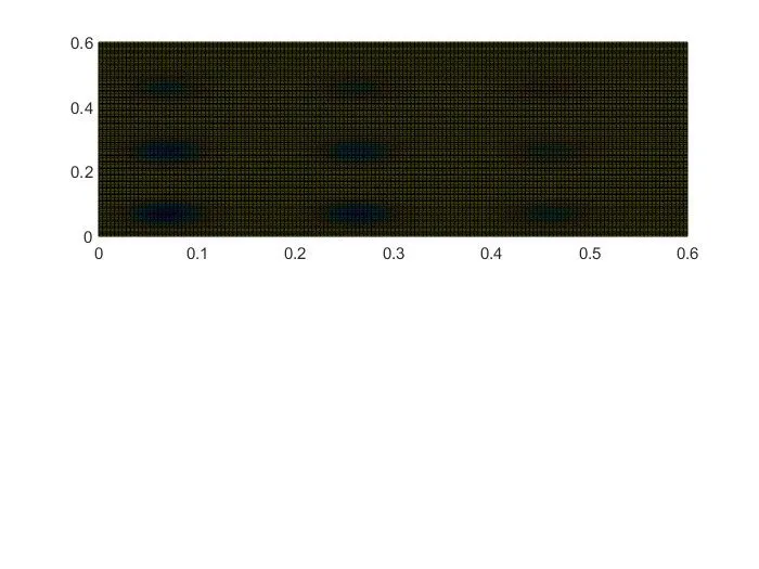
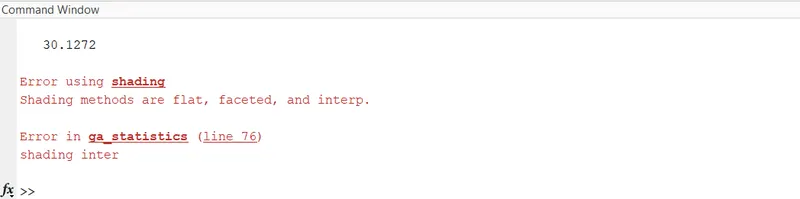
ERROR 1 - In study 3 instead of putting shading interp i put as shading inter so it gave wrong image as a plot.

ERROR 2 - In study 3 in options = optimoption command i put the value as 170 it gave me output with two values instead one exact value.

ERROR 3 - In stalagmite i forgot to add the negative symbol '-' in it so it gave me wrong plots and wrong minimum value.

ERROR REMEDIES

ERROR 1 - In command window I saw the error so i change that so error is neglected.

ERROR 2 - For this i don't have any idea about it so i make one-one session on that session i get the proper solution and i increase the value as 200 after that the error is gone.

ERROR 3 - For this also i don't know what to do so i make the one - one session in that session only i made a change in the function formula by adding '-' in it.

IMAGE OF ERRORS

ERROR 1

ERROR 2

ERROR 3