Week 4.1 - Genetic Algorithm
Aim:-
- Write a code in MATLAB to optimise the stalagmite function and find the global maxima of the function.
- Clearly expalin the concept of genetic algorithm in your own words and also explain the syntax for ga in MATLAB in your report.
- Make sure that your code gives the same output, even if it is made to run several times.
- Plot graphs for all 3 studies and for F maximum vs no. of iterations. Title and axes labels are a must, legends could be shown if necessary
Genetic Algorithm
The genetic algorithm is a method for solving both constrained and unconstrained optimization problems that is based on natural selection, the process that drives biological evolution. The genetic algorithm repeatedly modifies a population of individual solutions. At each step, the genetic algorithm selects individuals from the current population to be parents and uses them to produce the children for the next generation. Over successive generations, the population "evolves" toward an optimal solution. You can apply the genetic algorithm to solve a variety of optimization problems that are not well suited for standard optimization algorithms, including problems in which the objective function is discontinuous, nondifferentiable, stochastic, or highly nonlinear. The genetic algorithm can address problems of mixed integer programming, where some components are restricted to be integer-valued.
Basic process of solving problem with the help genetic algorithm
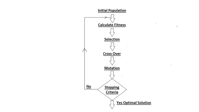
Optimization Problem
It is a theory and subject related to finding optimal point(refereing to maxima or minima). It can be used to solve both linear and non linear function.
Obiective Function
we have a non linear function = z that depends on variables like x and y;
z = f(x,y)
where f(x,y) = f1x*f2x*f1y*f2y
subjected to constraints
f1x = [sin(5.1pi*x+0.5)]^6
f2x = exp[-4ln(2)*(x-0.0667)^2/0.64]
f1y = [sin(5.1pi*y+0.5)]^6
f2y = exp[-4ln(2)*(y-0.0667)^2/0.64]
Solution
To solve above problem in MATLAB we will use Stalagmite function and 'ga' command.
Stalagmite function
Basically stalagmite represents the 3D pointed formations that arises from the floor like cones but may or may not be pointed always. In MATLAB, stalagmite function will generate a 3D figure of data of any function that will show us number of maximum points (local maxima) and number of minimum point (local minima). In optimization problem, we need to find most optimum points (i.e., global maxima or global minima) to rationalise our problem.
'ga' command
In MATLAB, 'ga' command is provided to solve optimization problem (i.e., stalagmite function) using genetic algorithm technique.
Steps to solve optimization function = z = f(x,y)
1. first we create a stalagmite function named = stal_func(input_vector)
function [z] = stal_func(input_veector)
x = input_veector(1);
y = input_veector(2);
2. Defining constraints
f1x = (sin(5.1*pi*x+0.5))^6;
f1y = (sin(5.1*pi*y+0.5))^6;
f2x = exp(-4*log(2).*(x-0.0667).^2/0.64);
f2y = exp(-4*log(2).*(y-0.0667).^2/0.64);
3. Providing optimization equation. Here negative sign is provded to balance the constraints.
z = -f1x*f2x*f1y*f2y;
end
MATLAB code for stalagmite function
function [z] = stal_func(input_veector)
x = input_veector(1);
y = input_veector(2);
f1x = (sin(5.1*pi*x+0.5))^6;
f1y = (sin(5.1*pi*y+0.5))^6;

f2x = exp(-4*log(2).*(x-0.0667).^2/0.64);
f2y = exp(-4*log(2).*(y-0.0667).^2/0.64);

z = -f1x*f2x*f1y*f2y;
end
Main program
1. first we will create an array of x and y
x = linspace(0,0.6,150);
y = linspace(0,0.6,150);
z = ones(size(y));
2. Here we have provided 100 cases to study
num_cases = 100;
3. Now we will use meshgrid command to create 2D mesh
[xx, yy] = meshgrid(x,y);
4. Than we will create loop to solve stalagmite function again and again 100 times. we have used for loop command for input i and j.
for i = 1:length(xx)
for j = 1:length(yy)
input_vector(1) = xx(i,j);
input_vector(2) = yy(i,j);
z(i,j) = stal_func(input_vector);
end
end
Study 1:-
Now we wil conduct our first study on each values of our optimation function (i.e., z). we will again create a loop to find a relation between our optimum values with respect to number of iterations(100). Also we will use 'tic-toc' command to find the time required to solve this iterations. then we will create a 3D plote of our results using 'surfc' command.
%study 1
tic
for i = 1:num_cases
[input,zopt(i)] = ga(@stal_func,2);
xopt(i) = input(1);
yopt(i) = input(2);
end
toc
figure (1)
subplot(2,1,1)
hold on
surfc(x,y,z);
shading interp;
plot3(xopt,yopt,zopt,'marker','o','MarkerSize',5,'Color','r');
title('Unbounded inputs');
subplot(2,1,2);
plot(zopt);
xlabel('Iteration');
ylabel('funtion Maxima');
Result:-
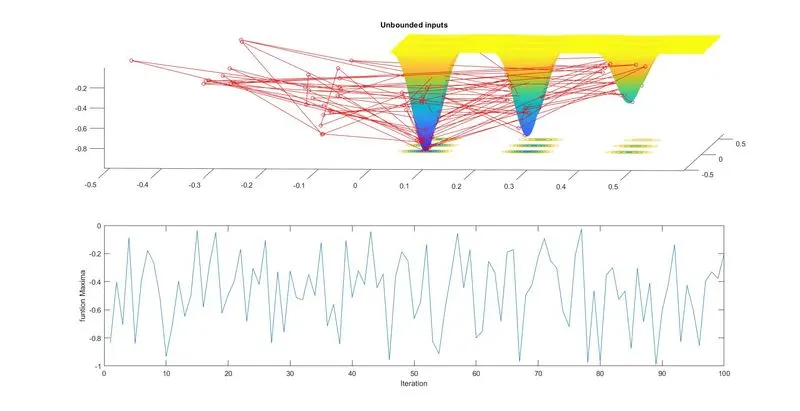
In study1 we get results of function z which is unbounded and spreaded beyond the ambit of our constraint points as shown in above figure.
Study 2:-
Now we wil conduct our second study on each values of our optimation function (i.e., z) within our contraint points. we will again create a loop to find a relation between our optimum values with respect to number of iterations(100). Also we will use 'tic-toc' command to find the time required to solve this iterations. then we will create a 3D plote of our results using 'surfc' command.
%study 2
tic
for i = 1:num_cases
[input,zopt(i)] = ga(@stal_func,2,[],[],[],[],[0;0],[1;1]);
xopt(i) = input(1);
yopt(i) = input(2);
end
toc
figure (2)
subplot(2,1,1)
hold on
surfc(x,y,z)
shading interp
plot3(xopt,yopt,zopt,'marker','o','MarkerSize',5,'Color','r');
title('Bounded inputs')
subplot(2,1,2);
plot(zopt);
xlabel('Iteration');
ylabel('funtion Maxima');
Result:-
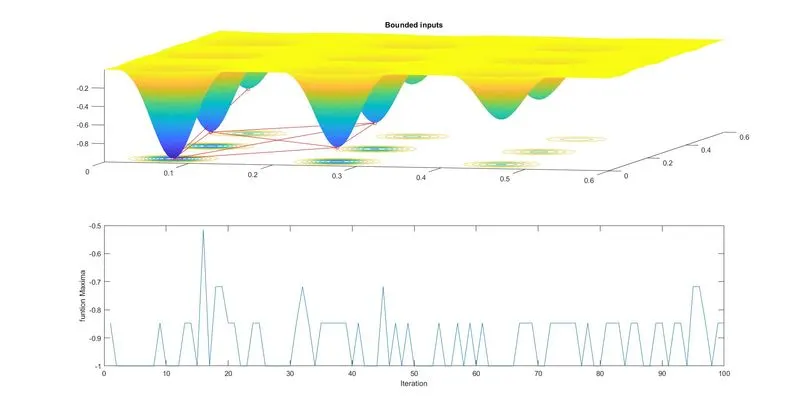
In study 2 we get optimum values within constraint points but it shows number of local maximas and minimas.
Study 3 :-
Now we wil conduct our third study on each values of our optimation function (i.e., z) to find most optimum (global maxima and minima). To find this will use 'optimoptions' to solve our 'ga' equation and also we will provide populaion size of 500. we will again create a loop to find a relation between our optimum values with respect to number of iterations(100). Also we will use 'tic-toc' command to find the time required to solve this iterations. then we will create a 3D plote of our results using 'surfc' command.
%study 3
options = optimoptions('ga');
options = optimoptions(options,'PopulationSize',500);
tic
for i = 1:num_cases
[input,zopt(i)] = ga(@stal_func,2,[],[],[],[],[0;0],[1;1],[],[],options);
xopt(i) = input(1);
yopt(i) = input(2);
end
toc
figure (3)
subplot(2,1,1)
hold on
surfc(x,y,z)
shading interp
plot3(xopt,yopt,zopt,'marker','d','MarkerSize',5,'Color','r');
title('Bounded inputs')
subplot(2,1,2);
plot(zopt);
xlabel('Iteration');
ylabel('funtion Maxima');
Reault :-
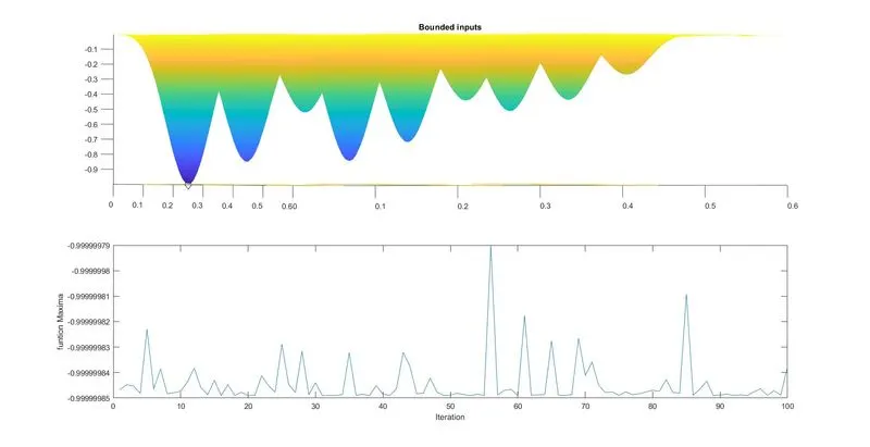
In study 3 we have find the most optmum values of function z which is maxima(z) = -0.99999979 and minimum(z) = -0.99999965
MATLA code for iterations
clear all
close all
clc
x = linspace(0,0.6,150);
y = linspace(0,0.6,150);
z = ones(size(y));
num_cases = 100;

[xx, yy] = meshgrid(x,y);

for i = 1:length(xx)
    for j = 1:length(yy)

        input_vector(1) = xx(i,j);
        input_vector(2) = yy(i,j);

        z(i,j) = stal_func(input_vector);
    end
end

%study 1

tic
for i = 1:num_cases
    [input,zopt(i)] = ga(@stal_func,2);
    xopt(i) = input(1);
    yopt(i) = input(2);
end
toc
figure (1)
subplot(2,1,1)
hold on

surfc(x,y,z);
shading interp;
plot3(xopt,yopt,zopt,'marker','o','MarkerSize',5,'Color','r');
title('Unbounded inputs');

subplot(2,1,2);
plot(zopt);
xlabel('Iteration');
ylabel('funtion Maxima');


%study 2
tic
for i = 1:num_cases
    [input,zopt(i)] = ga(@stal_func,2,[],[],[],[],[0;0],[1;1]);

    xopt(i) = input(1);
    yopt(i) = input(2);
end
toc
figure (2)
subplot(2,1,1)
hold on

surfc(x,y,z)
shading interp
plot3(xopt,yopt,zopt,'marker','o','MarkerSize',5,'Color','r');
title('Bounded inputs')

subplot(2,1,2);
plot(zopt);
xlabel('Iteration');
ylabel('funtion Maxima');

%study 3
options = optimoptions('ga');
options = optimoptions(options,'PopulationSize',500);
tic
for i = 1:num_cases
    [input,zopt(i)] = ga(@stal_func,2,[],[],[],[],[0;0],[1;1],[],[],options);

    xopt(i) = input(1);
    yopt(i) = input(2);
end
toc
figure (3)
subplot(2,1,1)
hold on

surfc(x,y,z)
shading interp
plot3(xopt,yopt,zopt,'marker','d','MarkerSize',5,'Color','r');
title('Bounded inputs')

subplot(2,1,2);
plot(zopt);
xlabel('Iteration');
ylabel('funtion Maxima');
Errors:-
Main error occur while running code is it shows inverted figure with resulted values point at the base as shown below
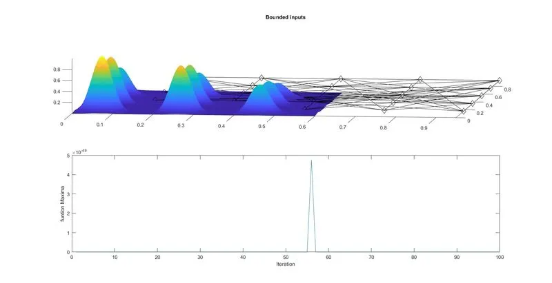
To overcome this issue i have to add a negative sign in objective function equation in stalagmite function code (i.e., z = -(f1x*f2x*f1y*f2y))