Project 1 - Parsing NASA thermodynamic data
Parsing NASA thermodynamic data
Aim:-
1. Write MATLAB code to extract thermodynamic data from the NASA thermodynamic data file and utilise to calculate thermodynamic properties of each Species(molecules) at given temperature range like Specific heat, Enthalpy, and Entropy.
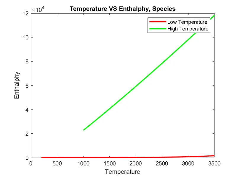
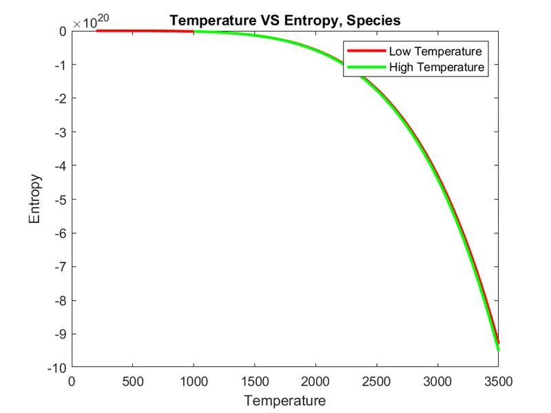
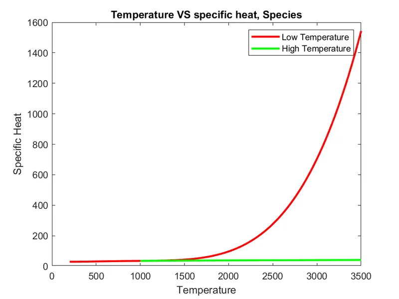
2. Also plot relation between temperature and thermodynamic properties and create individual folders for each species.
3. Also calculate molecular weight of each species and print their values in command window.
Solution:-
NASA has provided us polynomial relation to calculate thermodynamic properties :-

where cp = specific heat KJ/Kg K
H = Enthalpy KJ/Kg K
S = Entropy KJ/Kg K
Procedure:-
1. First we will create a folder where we will save our MATLAB code file and also we will move THERMO.dat file to this folder.
2. we will use 'fopen' command to open THERMO.dat file
f = fopen('THERMO.dat','r');
here 'r' represent read command
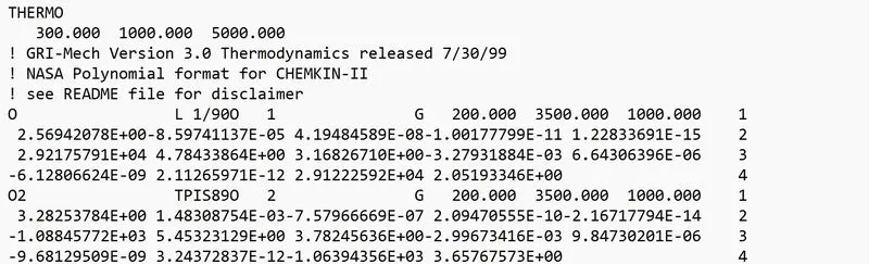
3. now we will use 'fgetl' command to read lines in THERMO.dat file
fgetl(f);
it will read => 'THERMO'
4. now we will use 'fgetl' command to read next line which is '300.000 1000.000 5000.000'
tline = fgetl(f);.
5. the above line is in string form and we have to convert it into numbers so we will use 'str2num' command
A = str2num(tline);
6. now we will show numbers in temperature form
global_low_temp = A(:,1);
global_mid_temp = A(:,2);
global_high_temp = A(:,3);
7.next three lines are comment line so we will skip these three lines
fgetl(f)
fgetl(f)
fgetl(f)
or we can use 'for loop' command
for i = 1:3
fgetl(f)
end
8. the next line represent our first specie which is oxygen (O) and local temperature ranges followed by next three line which provides us necessary values for the calculation thermodynamic properties of oxygen(O). And this pattern will we repeated till the last specie. so we will create here a loop command to work for all 53 species.
for i = 1:53
9. line1 will represent oxygen (O) line and we will use fgetl to read it
line1 = fgetl(f);
10. also this line1 is in string form and we need to convert it into charters and numbers, so we will use 'strsplit' command
l = strsplit(line1);
11. now we will use 'lenght' command to provide above line a length i.e., m = 10
m = length(l);
12. now we will define length = 1 = specie
sp = l(1);
13. now sp is in cell form and we need to convert it into scaler character so we will use 'char' command.
species = char(sp);
14. now we will define elements whose combination forms our species and also we will provide their atomic weight. this information will we utilise to calculate molecular weight
atom = ['H','C','O','N','Ar','S'];
atomic_weight = [1.008 12.011 15.999 14.007 39.948 32.065];
15. now we will read local temperature range in the line with the help of 'str2double' command
low_temp = str2double(l(m-3));
mid_temp = str2double(l(m-2));
high_temp = str2double(l(m-1));
16. now we will read next line with the help of 'fgetl' command and we will use 'strfind' command to find 'E' in the line so that we can easily provide coordinates of each values of 'a' based on 'E".
we will repeat same procedure for next two lines
line2 = fgetl(f);
a = strfind(line2,'E');
a1 = str2double(line2(1:(a+3)));
a2 = str2double(line2((a(1)+4):(a(2)+3)));
a3 = str2double(line2((a(2)+4):(a(3)+3)));
a4 = str2double(line2((a(3)+4):(a(4)+3)));
a5 = str2double(line2((a(4)+4):(a(5)+3)));
line3 = fgetl(f);
b = strfind(line3,'E');
a6 = str2double(line3(1:(b(1)+3)));
a7 = str2double(line3((b(1)+4):(a(2)+3)));
a8 = str2double(line3((b(2)+4):(a(3)+3)));
a9 = str2double(line3((b(3)+4):(a(4)+3)));
a10 = str2double(line3((b(4)+4):(a(5)+3)));
line4 = fgetl(f);
c = strfind(line3,'E');
a11 = str2double(line4(1:(c(1)+3)));
a12 = str2double(line4((c(1)+4):(a(2)+3)));
a13 = str2double(line4((c(2)+4):(a(3)+3)));
a14 = str2double(line4((c(3)+4):(a(4)+3)));
17. now we will create lower and higher temperature value array using 'linspace' command with interval of 100
%creating temperature values for lower and higher temperature
TL = linspace(low_temp,mid_temp,100);
TH = linspace(mid_temp,high_temp,100);
18. here we will define universal gas constant = R =8.314
R = 8.314;
19. now to calculate specific heat, enthalpy and entropy for lower and higher temperatures for each species, we will again create loop command.
for k = 1:100
%for lower temperature
cp_low(k) = (a8 + a9*TL(k) + a10*TL(k)^2 + a11*TL(k)^3 + a12*TL(k)^4)*R;
h_low(k) = (a8 + a9*TL(k)/2 + a10*(TL(k)^2)/3 + a11*(TL(k)^3)/4 + a12*(TL(k)^4)/5 + a13/TL(k))*R*TL(k);
s_low(k) = (a8*log(TL(k)) + a9*TL(k) + a10*(TL(k)^2)/2 + a11*(TL(k)^3)/3 + a12*(TL(k)^4)/4 + a13*(TL(k)^5)/5 +a14)*R;
%for higher temperature
cp_high(k) = (a1 + a2*TH(k) + a3*TH(k)^2 + a4*TH(k)^3 + a5*TH(k)^4)*R;
h_high(k) = (a1 + a2*TH(k)/2 + a3*TH(k)^2/3 + a4*TH(k)^3/4 + a5*TH(k)^4/5 + a6/TH(k))*R*TH(k);
s_high(k) = (a1*log(TH(k)) + a2*TH(k) + a3*TH(k)^2/2 + a4*TH(k)^3/3 + a5*TH(k)^4/4 + a6*TH(k)^5/5 +a7)*R;
end
20. now to save each plot of thermodynamic properties of each specie with repect to themperature range in an individual specie folder we will use 'mkdir' command
nasa_file = species;
mkdir(nasa_file);
current = pwd;
cd(nasa_file);
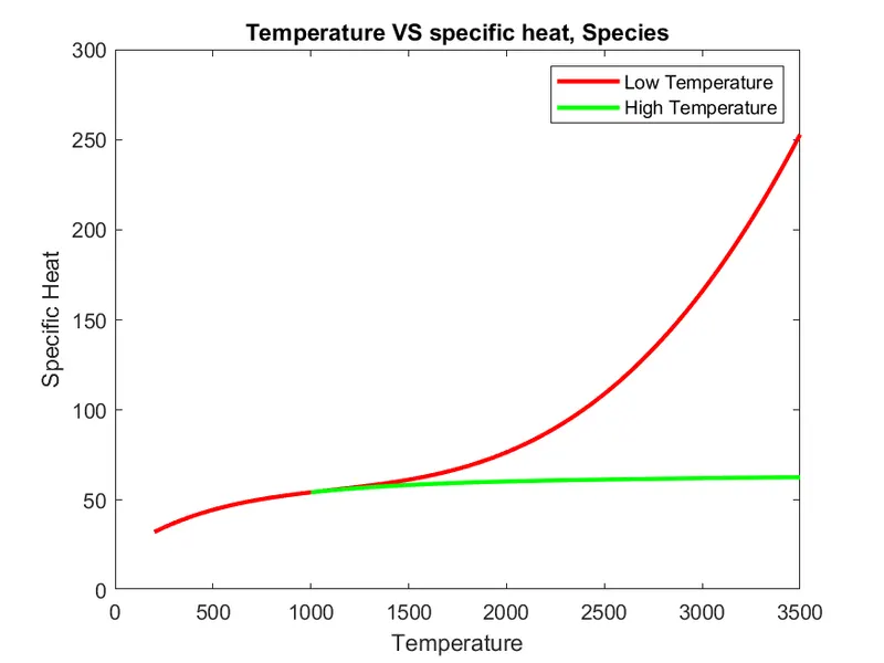
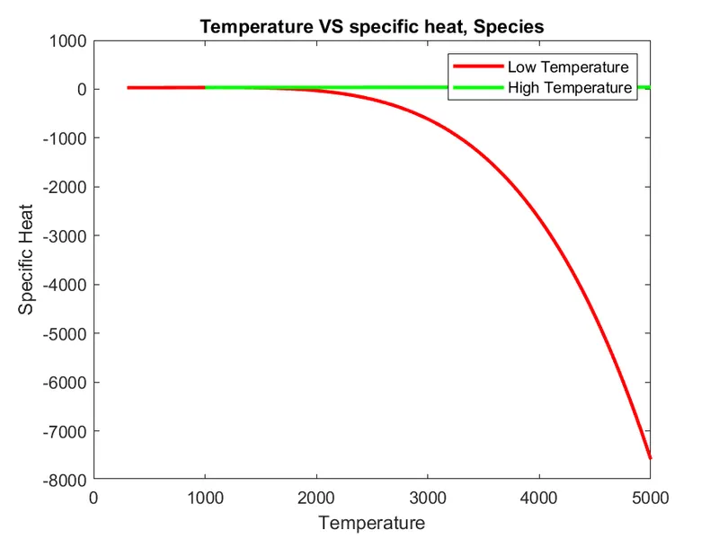
21. following command is use to create plot of specific heat vs temperature
%creating figure of specific heat
figure(1)
plot(TL,cp_low,'LineWidth',2,'color','r');
hold on
plot(TH,cp_high,'LineWidth',2,'Color','g');
hold off
title(['Temperature VS specific heat, Species']);
xlabel('Temperature');
ylabel('Specific Heat');
legend('Low Temperature','High Temperature');
% saving .png file of figure
fig = sprintf('specific heat of %s.png',species);
saveas(gca,fig);
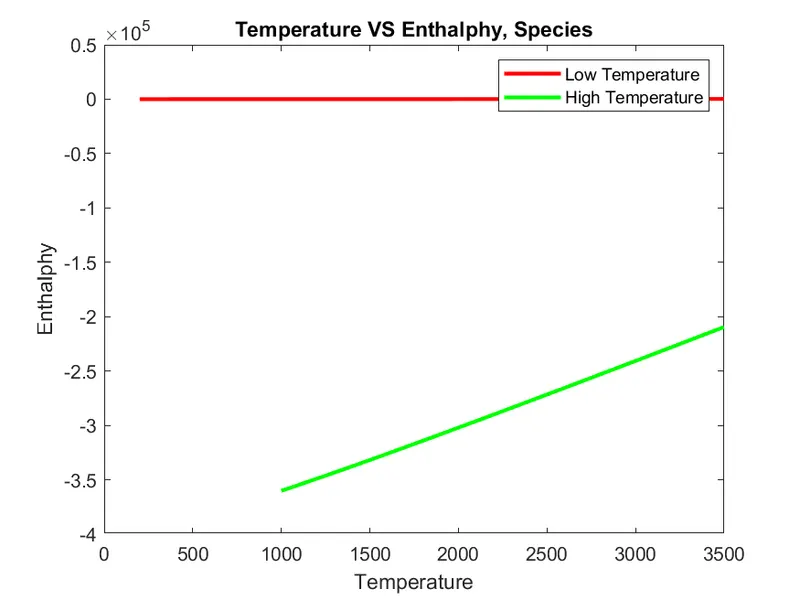
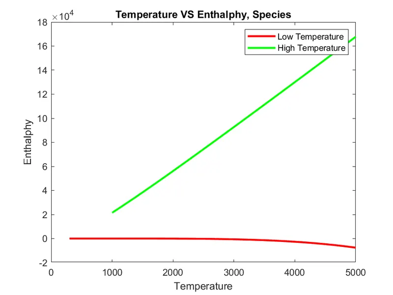
22. following command is use to create plot of enthaply vs temperature
%creating figure of enthalpy
figure(2)
plot(TL,cp_low,'LineWidth',2,'color','r');
hold on
plot(TH,h_high,'LineWidth',2,'Color','g');
hold off
title(['Temperature VS Enthalphy, Species']);
xlabel('Temperature');
ylabel('Enthalphy');
legend('Low Temperature','High Temperature');
% saving .png file of figure
fig = sprintf('enthalpy of %s.png',species);
saveas(gca,fig);
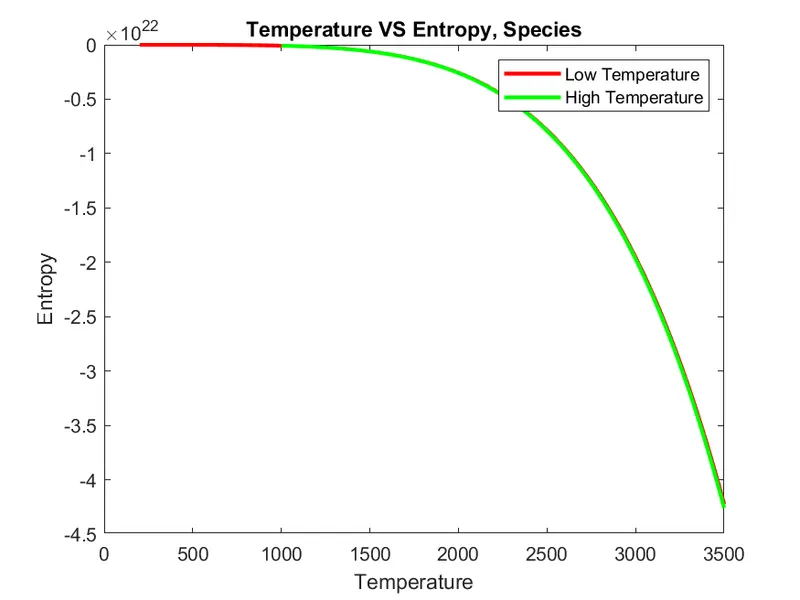
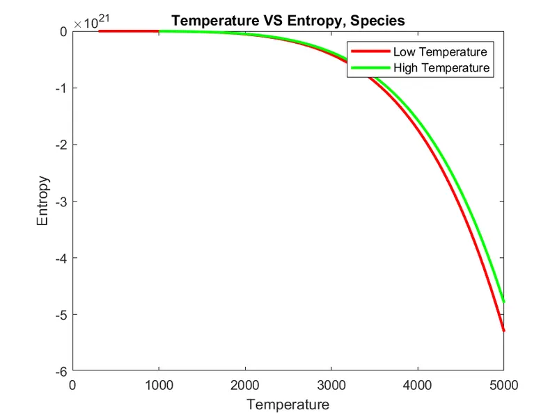
23. following command is use to create plot of entropy vs temperature
%creating figure of entropy
figure(3)
plot(TL,s_low,'LineWidth',2,'color','r');
hold on
plot(TH,s_high,'LineWidth',2,'Color','g');
hold off
title(['Temperature VS Entropy, Species']);
xlabel('Temperature');
ylabel('Entropy');
legend('Low Temperature','High Temperature');
% saving .png file of figure
fig = sprintf('entropy of %s.png',species);
saveas(gca,fig);
cd(current);
24. now to calculate molecular weight = mw of each specie. Here we again use loop command.
mw = 0;
for p = 1 : length(species)
for q = 1 : length(atomic_weight)
if strcmp(species(p),atom(q))
mw = mw + atomic_weight(q);
position = q;
end
end
%used for multiplication into the number of atoms
n = str2double(species(p));
if n>1
mw = mw + atomic_weight(position)*(n-1);
end
end
25. to display molecular weight of each species we will use 'fprintf' command
fprintf('molecular weight of %s : %f\n',species,mw);
end
clc
close all
clear all

%geting data file
f = fopen('THERMO.dat','r');
fgetl(f);

%reading header informations
tline = fgetl(f);
A = str2num(tline);
global_low_temp = A(:,1);
global_mid_temp = A(:,2);
global_high_temp = A(:,3);

%skipping comment lines
for i = 1:3
    fgetl(f)
end

%reading species data
for i = 1:53
line1 = fgetl(f);
l = strsplit(line1);
m = length(l);
sp = l(1);
species = char(sp);
atom = ['H','C','O','N','Ar','S'];
atomic_weight = [1.008 12.011 15.999 14.007 39.948 32.065];

low_temp = str2double(l(m-3));
mid_temp = str2double(l(m-2));
high_temp = str2double(l(m-1));

%storing the value of second line
line2 = fgetl(f);
a = strfind(line2,'E');
a1 = str2double(line2(1:(a+3)));
a2 = str2double(line2((a(1)+4):(a(2)+3)));
a3 = str2double(line2((a(2)+4):(a(3)+3)));
a4 = str2double(line2((a(3)+4):(a(4)+3)));
a5 = str2double(line2((a(4)+4):(a(5)+3)));

%storing the value of 3rd line

line3 = fgetl(f);
b = strfind(line3,'E');
a6 = str2double(line3(1:(b(1)+3)));
a7 = str2double(line3((b(1)+4):(a(2)+3)));
a8 = str2double(line3((b(2)+4):(a(3)+3)));
a9 = str2double(line3((b(3)+4):(a(4)+3)));
a10 = str2double(line3((b(4)+4):(a(5)+3)));

%storing the value of 4th line
line4 = fgetl(f);
c = strfind(line3,'E');
a11 = str2double(line4(1:(c(1)+3)));
a12 = str2double(line4((c(1)+4):(a(2)+3)));
a13  = str2double(line4((c(2)+4):(a(3)+3)));
a14 = str2double(line4((c(3)+4):(a(4)+3)));

%creating temperature values for lower and higher temperature
TL = linspace(low_temp,mid_temp,100);
TH = linspace(mid_temp,high_temp,100);

%value of universal gas constant
R = 8.314;


%calculating specific heat, enthalpy and entropy for lower and higher temperature
 for k = 1:100
%for lower temperature
cp_low(k) = (a8 + a9*TL(k) + a10*TL(k)^2 + a11*TL(k)^3 + a12*TL(k)^4)*R;
h_low(k) = (a8 + a9*TL(k)/2 + a10*(TL(k)^2)/3 + a11*(TL(k)^3)/4 + a12*(TL(k)^4)/5 + a13/TL(k))*R*TL(k);
s_low(k) = (a8*log(TL(k)) + a9*TL(k) + a10*(TL(k)^2)/2 + a11*(TL(k)^3)/3 + a12*(TL(k)^4)/4 + a13*(TL(k)^5)/5 +a14)*R;
%for higher temperature
cp_high(k) = (a1 + a2*TH(k) + a3*TH(k)^2 + a4*TH(k)^3 + a5*TH(k)^4)*R;
h_high(k) = (a1 + a2*TH(k)/2 + a3*TH(k)^2/3 + a4*TH(k)^3/4 + a5*TH(k)^4/5 + a6/TH(k))*R*TH(k);
s_high(k) = (a1*log(TH(k)) + a2*TH(k) + a3*TH(k)^2/2 + a4*TH(k)^3/3 + a5*TH(k)^4/4 + a6*TH(k)^5/5 +a7)*R;


end
   %creating folder
 nasa_file = species;
 mkdir(nasa_file);
 current = pwd;
 cd(nasa_file);

 %creating figure of specific heat
  figure(1)
  plot(TL,cp_low,'LineWidth',2,'color','r');
  hold on
  plot(TH,cp_high,'LineWidth',2,'Color','g');
  hold off
  title(['Temperature VS specific heat, Species']);
  xlabel('Temperature');
  ylabel('Specific Heat');
  legend('Low Temperature','High Temperature');

  % saving .png file of figure
  fig = sprintf('specific heat of %s.png',species);
  saveas(gca,fig);

  %creating figure of enthalpy
  figure(2)
  plot(TL,cp_low,'LineWidth',2,'color','r');
  hold on
  plot(TH,h_high,'LineWidth',2,'Color','g');
  hold off
  title(['Temperature VS Enthalphy, Species']);
  xlabel('Temperature');
  ylabel('Enthalphy');
  legend('Low Temperature','High Temperature');

  % saving .png file of figure
  fig = sprintf('enthalpy of %s.png',species);
  saveas(gca,fig);

  %creating figure of entropy
  figure(3)
  plot(TL,s_low,'LineWidth',2,'color','r');
  hold on
  plot(TH,s_high,'LineWidth',2,'Color','g');
  hold off
  title(['Temperature VS Entropy, Species']);
  xlabel('Temperature');
  ylabel('Entropy');
  legend('Low Temperature','High Temperature');

  % saving .png file of figure
  fig = sprintf('entropy of %s.png',species);
  saveas(gca,fig);
  cd(current);

  %calculation of molecular weight
atom = ['H','C','O','N','Ar','S'];
atomic_weight = [1.008 12.011 15.999 14.007 39.948 32.065];
mw = 0;

for p = 1 : length(species)
for q = 1 : length(atomic_weight)
if strcmp(species(p),atom(q))
mw = mw + atomic_weight(q);
position = q;
end
end
%used for multiplication into the number of atoms
n = str2double(species(p));
if n>1
mw = mw + atomic_weight(position)*(n-1);
end
end

 %display molecular weight.

fprintf('molecular weight of %s : %f\n',species,mw);

end
Results:-
1. Molecular weight of each specie
molecular weight of O : 15.999000
molecular weight of O2 : 31.998000
molecular weight of H : 1.008000
molecular weight of H2 : 2.016000
molecular weight of OH : 17.007000
molecular weight of H2O : 18.015000
molecular weight of HO2 : 33.006000
molecular weight of H2O2 : 34.014000
molecular weight of C : 12.011000
molecular weight of CH : 13.019000
molecular weight of CH2 : 14.027000
molecular weight of CH2(S) : 14.027000
molecular weight of CH3 : 15.035000
molecular weight of CH4 : 16.043000
molecular weight of CO : 28.010000
molecular weight of CO2 : 44.009000
molecular weight of HCO : 29.018000
molecular weight of CH2O : 30.026000
molecular weight of CH2OH : 31.034000
molecular weight of CH3O : 31.034000
molecular weight of CH3OH : 32.042000
molecular weight of C2H : 25.030000
molecular weight of C2H2 : 26.038000
molecular weight of C2H3 : 27.046000
molecular weight of C2H4 : 28.054000
molecular weight of C2H5 : 29.062000
molecular weight of C2H6 : 30.070000
molecular weight of CH2CO : 42.037000
molecular weight of HCCO : 41.029000
molecular weight of HCCOH : 42.037000
molecular weight of H2CN : 28.034000
molecular weight of HCN : 27.026000
molecular weight of HNO : 31.014000
molecular weight of N : 14.007000
molecular weight of NNH : 29.022000
molecular weight of N2O : 44.013000
molecular weight of NH : 15.015000
molecular weight of NH2 : 16.023000
molecular weight of NH3 : 17.031000
molecular weight of NO : 30.006000
molecular weight of NO2 : 46.005000
molecular weight of HCNO : 43.025000
molecular weight of HOCN : 43.025000
molecular weight of HNCO : 43.025000
molecular weight of NCO : 42.017000
molecular weight of CN : 26.018000
molecular weight of HCNN : 41.033000
molecular weight of N2 : 28.014000
molecular weight of AR : 39.948000
molecular weight of C3H8 : 44.097000
molecular weight of C3H7 : 43.089000
molecular weight of CH3CHO : 44.053000
molecular weight of CH2CHO : 43.045000
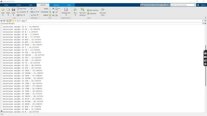
2. Screenshot of the window where all the folders are saved.

3. Plots for o2
4. Plots for N2
5. Plots for Co2