Week 3 - Solving second order ODEs
Aim:- To Solve second order Ordinary Differential Equation (ODE)
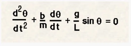
Write a program in Matlab\Octave that will simulate the pendulum motion, just like the one shown in the start of this challenge.
L=1 metre,
m=1 kg,
b=0.05.
g=9.81 m/s2.
Simulate the motion between 0-20 sec, for angular displacement=0,angular velocity=3 rad/sec at time t=0.
MATLAB Codings.
1. First of all to solve the various values of theta with respect to time, we will use 'function' command
1. now we will create a function = [dth_dt]
where th = theta
dth_dt = differential of theta with respect to time
function [dth_dt] = ODE_pendulum(t,th,b,g,l,m)
th1 = th(1); %theta1 = th1
th2 = th(2); %theta2 = th2
dth1_dt = th2;
dth2_dt = -(b/m) * th2 - (g/l) * sin(th1);
dth_dt = [dth1_dt;dth2_dt];
end
MATLAB codings:-
function [dth_dt] = ODE_pendulum(t,th,b,g,l,m)
th1 = th(1); %theta1 = th1
th2 = th(2); %theta2 = th2
dth1_dt = th2;
dth2_dt = -(b/m) * th2 - (g/l) * sin(th1);
dth_dt = [dth1_dt;dth2_dt];
end
2. Codes for the calculation of ODE
1. inputs conditions
g = 9.81;
l = 1;
b = 0.05;
m = 1;
2. program to simulate motion
%initial conditions => at angular displacement = 0 => velocity = 3rad/sec => theta_0
th_0 = [0;3];
3. time array => motion between 0 to 20 sec with 500 divisions
t_span = linspace(0,20,500);
4. To ODE in MATLAB we use 'ode45' command
in the following program, command is used to find matrix [time results(differential values of theta with respect to time]
[t,results] = ode45(@(t,th)ODE_pendulum(t,th,b,g,l,m),t_span,th_0);
5. To plot our result in separate graphs of angular displacement and angular velocity
figure(1)
subplot(2,1,1);
plot(t,results(:,1),'color','g');
xlabel('time');
ylabel(' angular displacement')
title('Angular Quantities as afunction of time');
subplot(2,1,2);
plot(t,results(:,2),'color','m');
xlabel('time');
ylabel('angular velocity ');
grid on
MATLAB codings:-
%inputs
g = 9.81;
l = 1;
b = 0.05;
m = 1;

%program to simulate motion
%initial conditions => at angular displacement = 0 => velocity = 3rad/sec
%=> theta_0
th_0 = [0;3];

% time array => motion between 0 to 20 sec with 500 divisions
t_span = linspace(0,20,500);

% solving ODE
[t,results] = ode45(@(t,th)ODE_pendulum(t,th,b,g,l,m),t_span,th_0);

% plots
figure(1)

subplot(2,1,1);
plot(t,results(:,1),'color','g');
xlabel('time');
ylabel(' angular displacement')
title('Angular Quantities as afunction of time');

subplot(2,1,2);
plot(t,results(:,2),'color','m');
xlabel('time');
ylabel('angular velocity ');

grid on

figure(2)

plot(t,results(:,1),'color','g');

title('Angular Quantities as afunction of time');
hold on
plot(t,results(:,2),'color','m');
xlabel('time');
ylabel('angular velocity and angular displacement');
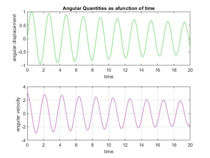
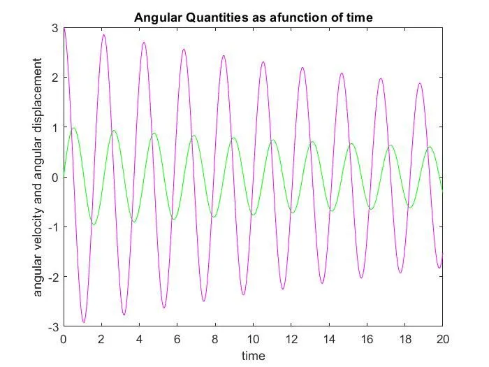
6. To plot our result in combined graphs of angular displacement and angular velocity
figure(2)
plot(t,results(:,1),'color','g');
title('Angular Quantities as afunction of time');
hold on
plot(t,results(:,2),'color','m');
xlabel('time');
ylabel('angular velocity and angular displacement');
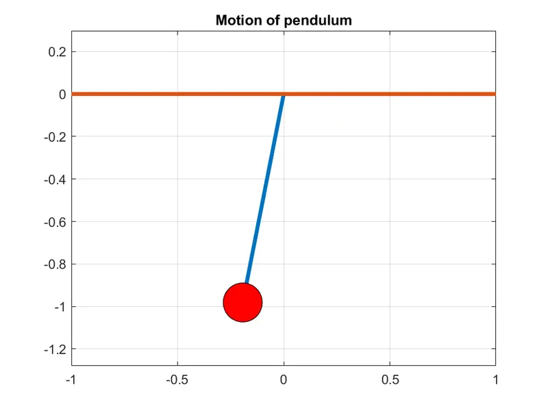
3. Code for the generation of animation of pendulum motion
Note :- I have done a separete coding for the creation of animation to reduce the chances of error in frames but we can also create a single code too by simply putting codes from % pendulum motion animation to close(videofile) in above codes
1. initial values
%inputs
g = 9.81;
l = 1;
b = 0.05;
m = 1;
%program to simulate motion
%initial conditions => at angular displacement = 0 => velocity = 3rad/sec
%=> theta_0
th_0 = [0;3];
% time array => motion between 0 to 20 sec with 500 divisions
t_span = linspace(0,20,500);
% solving ODE
[t,results] = ode45(@(t,th)ODE_pendulum(t,th,b,g,l,m),t_span,th_0);
for plotting the initial position of pendulum
% pendulum motion animation
figure(ct)
x0 = 0;
y0 = 0;
ct = 1;
we are using 'for loop' command here to create a motion matrix
for i = 1:length(t_span)
x1 = 1*sin((pi/20)-results(i));
y1 = -1*cos((pi/20)-results(i));
here we are plotting the position of cable
plot([x0 x1],[y0 y1],[-1 1],[0 0],'LineWidth',3);
hold on
here we are creating ball which is attacted with the above cable by using marker command
plot(x1,y1,'Marker','o','MarkerSize',30,'MarkerFaceColor','r','MarkerEdgeColor','k');
axis(gca,'equal');
title('Motion of pendulum')
grid on
pause(0.1)
ct = ct+1;
hold off
to create animation file following commads have provided
N(ct) = getframe(gcf);
end
Movie(N)
videofile = VideoWriter('pendulum7.avi','Uncompressed AVI');
open(videofile)
writeVideo(videofile,N)
close(videofile)
MATLAB codings:-
clear all
close all
clc

%inputs
g = 9.81;
l = 1;
b = 0.05;
m = 1;

%program to simulate motion
%initial conditions => at angular displacement = 0 => velocity = 3rad/sec
%=> theta_0
th_0 = [0;3];

% time array => motion between 0 to 20 sec with 500 divisions
t_span = linspace(0,20,500);

% solving ODE
[t,results] = ode45(@(t,th)ODE_pendulum(t,th,b,g,l,m),t_span,th_0);

% pendulum motion animation
 ct = 1;
figure(ct)
x0 = 0;
    y0 = 0;


for i = 1:length(t_span)


    x1 = 1*sin((pi/20)-results(i));
    y1 = -1*cos((pi/20)-results(i));


    plot([x0 x1],[y0 y1],[-1 1],[0 0],'LineWidth',3);
    hold on
    plot(x1,y1,'Marker','o','MarkerSize',30,'MarkerFaceColor','r','MarkerEdgeColor','k');

    axis(gca,'equal');
    title('Motion of pendulum')
    grid on
    pause(0.1)

    ct = ct+1;
    hold off
    M(i) = getframe(gcf);

end


videofile = VideoWriter('pendulum7.avi','Uncompressed AVI');
open(videofile)
writeVideo(videofile,M)
close(videofile)
Video file on youtube
ERROR occure during codings
while using following codings for the creation of animation :-
M(ct) = getframe(gcf);

end

movie(M)
videofile = VideoWriter('pendulum8.avi','Uncompressed AVI');
open(videofile)
writeVideo(videofile,M)
close(videofile)
i have encountered with following error
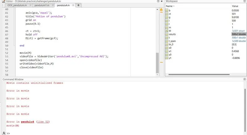
To resolve this issue i have replaced above coding with following
 M(i) = getframe(gcf);

end


videofile = VideoWriter('pendulum8.avi','Uncompressed AVI');
open(videofile)
writeVideo(videofile,M)
close(videofile)