Project 2 - Rankine cycle Simulator
Project 2 - Rankine cycle Simulator
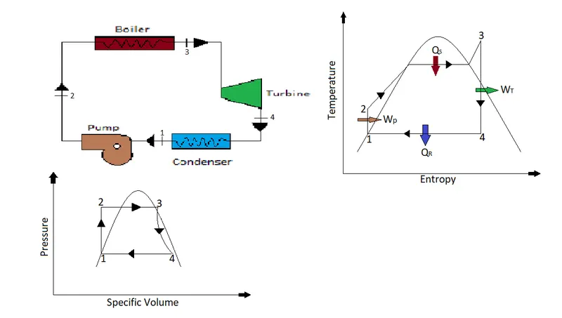
Rankine cycle is the practical working cycle for thermal power plant and it consist of four processes
Process 1-2 Reversible adiabatic compression process of feed water through feed pump.
Process 2-3 Constant pressure heat addition process in boiler.
Process 3-4 Reversible adiabatic expansion process of steam in turbine.
Process 4-1 Constant pressure heat rejection process in heat exchanger/condensor.
Aim:-
- Create a Rankine Cycle Simulator using OCTAVE/MATLAB.
- Calculate the state points of the Rankine Cycle (any type of your choice) based on user inputs.
- Plot the corresponding T-s and h-s plots for the given set of inputs.
Given:-
Turbine Inlet temperature = 400° C
Turbine Inlet Pressure = 30 bars
Turbine Outlet Pressure = 0.05 bars = Condenser Inlet Pressure
Calculate the followings:-
- Net work output
- Back work ratio
Calculation:-
Process 1-2 Reversible adiabatic compression process of feed water through feed pump.
Work Done on the system
Pump work = Wp = specific volume of saturated fluid x change in pressure from 1 to 2
Wp = (spv)f x dp = (spv)f x (pressure of fluid at inlet of boiler - pressure of fluid at outlet of condenser)
Wp = (spv)f x (P2 - P1) = (h2-h1) KJ/Kg of steam
Heat transfer
One unit of heat is the amount of heat requried to raise the temperature of one gram of fluid through one degree by keeping the pressure constant throughout.
Heat transfer = Q = mass of fluid x specific heat of fluid x change in temperature
Q = m x cp x dt KJ
for adiabatic process heat transfer is zero
Qp = 0
Process 2-3 Constant pressure heat addition process in boiler.
Work done in the process is zero as volume of boiler is fix (not changing)
Wb = presuure at the inlet of boiler x change of volume in boiler = 0
Heat supplied in the boiler
Heat transfer = Q = mass of fluid x specific heat of fluid x change in temperature
Q = m x cp x dt KJ
for 2 - 3 process heat is supplied to the system
Qs = m x (cp)f x (t3 - t2) KJ
Qs = m x (h3 - h2) KJ
Specific heat
qs = (h3 - h2) KJ/Kg
Process 3-4 Reversible adiabatic expansion process of steam in turbine.
Work done by the turbine
Turbine work = Wt = specific volume of saturated steam x change in pressure from 3 to 4
Wt = (spv)s x dp = (spv)s x (pressure of steam at the inlet of turbine - pressure of steam at the outlet of turbine)
Wt = (spv)s x (P3 - P4) = (h3-h4) KJ/Kg of steam
Heat transfer
Heat transfer = Q = mass of steam x specific heat of steam x change in temperature
Q = m x cp x dt KJ
for adiabatic process heat transfer is zero
Qp = 0
Process 4-1 Constant pressure heat rejection process in heat exchanger/condensor.
Work done in the process is zero as volume of condenser is fix (not changing)
Wc = presuure at the inlet of condenser x change of volume in boiler = 0
Heat Rejection in condenser
Heat transfer = Q = mass of steam x specific heat of steam x change in temperature
Q = m x cp x dt KJ
for 4 - 1 process heat is supplied to the system
Qc = m x (cp)g x (t4 - t1) KJ
Qc = m x (h4 - h1) kJ
Specific heat
qc = (h4 - h1) KJ/Kg
Net work
Wnet = turbine work - pump work
Wnet = Wt - Wp
Thermal efficiency of the system
eff = net work/heat supplied
eff = Wnet/Qs = (Wt - Wp)/Qs
Back work ratio
The ratio of the pump work to the turbine work is called the back-work ratio
Rb = Wp/Wt
MATLAB coding explainations
1. First we load XSteam function file.It will help to find out the values of various propertis of water in different state.It is like a steam table.
Method for calling XSteam function described in XSteam function file
% First the wanted property then a _ then the wanted input properties.
% Example. T_ph is temperature as a function of pressure and enthalpy.
% For a list of valid functions se bellow or XSteam for MS Excel.
% T Temperature (deg C)
% p Pressure (bar)
% h Enthalpy (kJ/kg)
% v Specific volume (m3/kg)
% rho Density
% s Specific entropy
% u Specific internal energy
% Cp Specific isobaric heat capacity
% Cv Specific isochoric heat capacity
% w Speed of sound
% my Viscosity
% tc Thermal Conductivity
% st Surface Tension
% x Vapour fraction
% vx Vapour Volume Fraction
%
%*** Valid Steam table functions. ****************************************************************************
%
%Temperature
%Tsat_p Saturation temperature
%T_ph Temperture as a function of pressure and enthalpy
%T_ps Temperture as a function of pressure and entropy
%T_hs Temperture as a function of enthalpy and entropy
%
%Pressure
%psat_T Saturation pressure
%p_hs Pressure as a function of h and s.
%p_hrho Pressure as a function of h and rho. Very unaccurate for solid water region since it's almost incompressible!
%
%Enthalpy
%hV_p Saturated vapour enthalpy
%hL_p Saturated liquid enthalpy
%hV_T Saturated vapour enthalpy
%hL_T Saturated liquid enthalpy
%h_pT Entalpy as a function of pressure and temperature.
%h_ps Entalpy as a function of pressure and entropy.
%h_px Entalpy as a function of pressure and vapour fraction
%h_prho Entalpy as a function of pressure and density. Observe for low temperatures (liquid) this equation has 2 solutions.
%h_Tx Entalpy as a function of temperature and vapour fraction
%
%Specific volume
%vV_p Saturated vapour volume
%vL_p Saturated liquid volume
%vV_T Saturated vapour volume
%vL_T Saturated liquid volume
%v_pT Specific volume as a function of pressure and temperature.
%v_ph Specific volume as a function of pressure and enthalpy
%v_ps Specific volume as a function of pressure and entropy.
%
%Density
%rhoV_p Saturated vapour density
%rhoL_p Saturated liquid density
%rhoV_T Saturated vapour density
%rhoL_T Saturated liquid density
%rho_pT Density as a function of pressure and temperature.
%rho_ph Density as a function of pressure and enthalpy
%rho_ps Density as a function of pressure and entropy.
%
%Specific entropy
%sV_p Saturated vapour entropy
%sL_p Saturated liquid entropy
%sV_T Saturated vapour entropy
%sL_T Saturated liquid entropy
%s_pT Specific entropy as a function of pressure and temperature (Returns saturated vapour entalpy if mixture.)
%s_ph Specific entropy as a function of pressure and enthalpy
%
%Specific internal energy
%uV_p Saturated vapour internal energy
%uL_p Saturated liquid internal energy
%uV_T Saturated vapour internal energy
%uL_T Saturated liquid internal energy
%u_pT Specific internal energy as a function of pressure and temperature.
%u_ph Specific internal energy as a function of pressure and enthalpy
%u_ps Specific internal energy as a function of pressure and entropy.
%
%Specific isobaric heat capacity
%CpV_p Saturated vapour heat capacity
%CpL_p Saturated liquid heat capacity
%CpV_T Saturated vapour heat capacity
%CpL_T Saturated liquid heat capacity
%Cp_pT Specific isobaric heat capacity as a function of pressure and temperature.
%Cp_ph Specific isobaric heat capacity as a function of pressure and enthalpy
%Cp_ps Specific isobaric heat capacity as a function of pressure and entropy.
%
%Specific isochoric heat capacity
%CvV_p Saturated vapour isochoric heat capacity
%CvL_p Saturated liquid isochoric heat capacity
%CvV_T Saturated vapour isochoric heat capacity
%CvL_T Saturated liquid isochoric heat capacity
%Cv_pT Specific isochoric heat capacity as a function of pressure and temperature.
%Cv_ph Specific isochoric heat capacity as a function of pressure and enthalpy
%Cv_ps Specific isochoric heat capacity as a function of pressure and entropy.
%
%Speed of sound
%wV_p Saturated vapour speed of sound
%wL_p Saturated liquid speed of sound
%wV_T Saturated vapour speed of sound
%wL_T Saturated liquid speed of sound
%w_pT Speed of sound as a function of pressure and temperature.
%w_ph Speed of sound as a function of pressure and enthalpy
%w_ps Speed of sound as a function of pressure and entropy.
%
%Viscosity
%Viscosity is not part of IAPWS Steam IF97. Equations from
%"Revised Release on the IAPWS Formulation 1985 for the Viscosity of Ordinary Water Substance", 2003 are used.
%Viscosity in the mixed region (4) is interpolated according to the density. This is not true since it will be two fases.
%my_pT Viscosity as a function of pressure and temperature.
%my_ph Viscosity as a function of pressure and enthalpy
%my_ps Viscosity as a function of pressure and entropy.
%
%Thermal Conductivity
%Revised release on the IAPS Formulation 1985 for the Thermal Conductivity of ordinary water substance (IAPWS 1998)
%tcL_p Saturated vapour thermal conductivity
%tcV_p Saturated liquid thermal conductivity
%tcL_T Saturated vapour thermal conductivity
%tcV_T Saturated liquid thermal conductivity
%tc_pT Thermal conductivity as a function of pressure and temperature.
%tc_ph Thermal conductivity as a function of pressure and enthalpy
%tc_hs Thermal conductivity as a function of enthalpy and entropy
%
%Surface tension
%st_T Surface tension for two phase water/steam as a function of T
%st_p Surface tension for two phase water/steam as a function of T
%Vapour fraction
%x_ph Vapour fraction as a function of pressure and enthalpy
%x_ps Vapour fraction as a function of pressure and entropy.
%
%Vapour volume fraction
%vx_ph Vapour volume fraction as a function of pressure and enthalpy
%vx_ps Vapour volume fraction as a function of pressure and entropy.
2. Now we will create a new .m file, and start coding.
3. Initially we provide input commands.
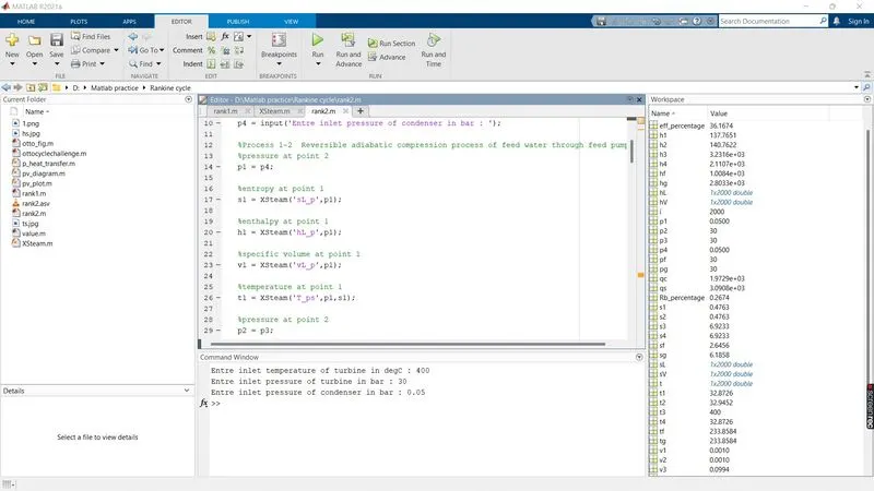
t3 = input('Entre inlet temperature of turbine in degC : ');
p3 = input('Entre inlet pressure of turbine in bar : ');
p4 = input('Entre inlet pressure of condenser in bar : ');
4.Now we will process wise codes
%Process 1-2 Reversible adiabatic compression process of feed water through feed pump.
%pressure at point 2
p1 = p4;
%entropy at point 1
s1 = XSteam('sL_p',p1);
%enthalpy at point 1
h1 = XSteam('hL_p',p1);
%specific volume at point 1
v1 = XSteam('vL_p',p1);
%temperature at point 1
t1 = XSteam('T_ps',p1,s1);
%pressure at point 2
p2 = p3;
%pressure at saturated liquid point
pf = p3;
%entropy at point 2
s2 = s1;
%entropy at saturated liquid point
sf = XSteam('sL_p',p2);
%temperature at point 2
t2 = XSteam('T_ps',p2,s2);
%temperature at saturated liquid point
tf = XSteam('Tsat_p',p2);
%enthalpy at point 2
h2 = XSteam('h_pT',p2,t2);
%enthalpy at saturated liquid point
hf = XSteam('hL_p',p2);
%specific volume at point 2
v2 = v1;
%specific volume at saturated liquid point
vf = XSteam('vL_p',p3);
%Process 2-3 Constant pressure heat addition process in boiler.
%temperature at saturated liquid point
tg = XSteam('Tsat_p',p3);
%pressure at saturated vapour point
pg = p3;
%entropy at point 3
s3 = XSteam('s_pT',p3,t3);
%entropy at saturated vapour
sg = XSteam('sV_p',p3);
%enthalpy at point 3
h3 = XSteam('h_ps',p3,s3);
%enthalpy at saturated liquid point
hg = XSteam('hV_p',p3);
%specific volume at point 3
v3 = XSteam('v_ps',p3,s3);
%specific volume at saturated liquid point
vg = XSteam('vV_p',p3);
%Process 3-4 Reversible adiabatic expansion process of steam in turbine.
%temperature at point 4
t4 = t1;
%entropy at point 4
s4 = s3;
%enthalpy at point 4
h4 = XSteam('h_ps',p4,s4);
%specific volume at point 4
v4 = XSteam('v_ps',p4,s4);
%Work Done on the system
Wp = (h2 - h1);
%heat supplied to the system
%qs = cp_f * (t3 - t2)
qs = (h3 - h2);
%Wt = spv_s * (P3 - P4)
Wt = (h3-h4);
%Process 4-1 Constant pressure heat rejection process in heat exchanger/condensor.
%Heat Rejection in condenser
%Qc = cp_g * (t4 - t1)
qc = (h4 - h1);
%Net work
%Wnet = turbine work - pump work
Wnet = Wt - Wp;
%Thermal efficiency of the system
%eff = net work/heat supplied
%eff = Wnet/Qs = (Wt - Wp)/Qs
eff_percentage = (Wt - Wp)/qs * 100 ;
%Back work ratio
%The ratio of the pump work to the turbine work is called the back-work ratio
Rb_percentage = Wp/Wt * 100;
%Ploting t-s , h-s and p-v plot
%ploting saturation lines
t = (1:2000);
for i = 1:1:2000
sL(1,i) = XSteam('sL_T',i);
sV(1,i) = XSteam('sV_T',i);
hL(1,i) = XSteam('hL_T',i);
hV(1,i) = XSteam('hV_T',i);
end
figure(1)
plot(sL,t,'b','linewidth',1);
hold on;
plot(sV,t,'b','linewidth',1);
xlabel('Entropy (KJ/Kg C)');
ylabel('Temperature (C)');
title('Temperature vs Entropy plot');
legend('Saturation curve');
figure(2)
plot(sL,hL,'b','linewidth',1);
hold on;
plot(sV,hV,'b','linewidth',1);
xlabel('Entropy (KJ/Kg C)');
ylabel('Enthalpy(KJ/Kg C)');
title('Enthalpy vs Entropy plot');
legend('Saturation curve');
%ploting Rankine Cycle
figure(1)
plot([s1,s2,sf,sg,s3,s4,s1],[t1,t2,tf,tg,t3,t4,t1],'k','linewidth',1);
text(s1,t1,'1');
text(s2,t2,'2');
text(sf,tf,'f');
text(sg,tg,'g');
text(s3,t3,'3');
text(s4,t4,'4');
figure(2)
plot([s1,s2,sf,sg,s3,s4,s1],[h1,h2,hf,hg,h3,h4,h1],'k','linewidth',1);
text(s1,h1,'1');
text(s2,h2,'2');
text(sf,hf,'f');
text(sg,hg,'g');
text(s3,h3,'3');
text(s4,h4,'4');
MATLAB Codes:-
clc
clear all
close all
% Given:-
%Turbine Inlet temperature = 400° C
%Turbine Inlet Pressure = 30 bars
%Turbine Outlet Pressure = 0.05 bars = Condenser Inlet Pressure
t3 = input('Entre inlet temperature of turbine in degC : ');
p3 = input('Entre inlet pressure of turbine in bar : ');
p4 = input('Entre inlet pressure of condenser in bar : ');

%Process 1-2  Reversible adiabatic compression process of feed water through feed pump.
%pressure at point 2
p1 = p4;

%entropy at point 1
s1 = XSteam('sL_p',p1);

%enthalpy at point 1
h1 = XSteam('hL_p',p1);

%specific volume at point 1
v1 = XSteam('vL_p',p1);

%temperature at point 1
t1 = XSteam('T_ps',p1,s1);

%pressure at point 2
p2 = p3;

%pressure at saturated liquid point
pf = p3;

%entropy at point 2
s2 = s1;

%entropy at saturated liquid point
sf = XSteam('sL_p',p2);

%temperature at point 2
t2 = XSteam('T_ps',p2,s2);

%temperature at saturated liquid point
tf = XSteam('Tsat_p',p2);

%enthalpy at point 2
h2 = XSteam('h_pT',p2,t2);

%enthalpy at saturated liquid point
hf = XSteam('hL_p',p2);

%specific volume at point 2
v2 = v1;

%specific volume at saturated liquid point
vf = XSteam('vL_p',p3);

%Process 2-3  Constant pressure heat addition process in boiler.
%temperature at saturated liquid point
tg = XSteam('Tsat_p',p3);

%pressure at saturated vapour point
pg = p3;

%entropy at point 3
s3 = XSteam('s_pT',p3,t3);

%entropy at saturated vapour
sg = XSteam('sV_p',p3);

%enthalpy at point 3
h3 = XSteam('h_ps',p3,s3);

%enthalpy at saturated liquid point
hg = XSteam('hV_p',p3);

%specific volume at point 3
v3 = XSteam('v_ps',p3,s3);

%specific volume at saturated liquid point
vg = XSteam('vV_p',p3);

%Process 3-4  Reversible adiabatic expansion process of steam in turbine.
%temperature at point 4
t4 = t1;

%entropy at point 4
s4 = s3;

%enthalpy at point 4
h4 = XSteam('h_ps',p4,s4);

%specific volume at point 4
v4 = XSteam('v_ps',p4,s4);

%Work Done on the system
Wp = (h2 - h1);

%heat supplied to the system
%qs = cp_f * (t3 - t2)
qs = (h3 - h2);

%Wt = spv_s * (P3 - P4)
Wt = (h3-h4);

%Process 4-1  Constant pressure heat rejection process in heat exchanger/condensor.
%Heat Rejection in condenser
%Qc = cp_g * (t4 - t1)
qc = (h4 - h1);

%Net work
%Wnet = turbine work - pump work
Wnet = Wt - Wp;

%Thermal efficiency of the system
%eff = net work/heat supplied
%eff = Wnet/Qs = (Wt - Wp)/Qs
eff_percentage = (Wt - Wp)/qs * 100 ;

%Back work ratio
%The ratio of the pump work to the turbine work is called the back-work ratio
Rb_percentage = Wp/Wt * 100;

%Ploting t-s , h-s and p-v plot
%ploting saturation lines
t = (1:2000);
for i = 1:1:2000
    sL(1,i) = XSteam('sL_T',i);
    sV(1,i) = XSteam('sV_T',i);
    hL(1,i) = XSteam('hL_T',i);
    hV(1,i) = XSteam('hV_T',i);
end

figure(1)
plot(sL,t,'b','linewidth',1);
hold on;
plot(sV,t,'b','linewidth',1);
xlabel('Entropy (KJ/Kg C)');
ylabel('Temperature (C)');
title('Temperature vs Entropy plot');
legend('Saturation curve');

figure(2)
plot(sL,hL,'b','linewidth',1);
hold on;
plot(sV,hV,'b','linewidth',1);
xlabel('Entropy (KJ/Kg C)');
ylabel('Enthalpy(KJ/Kg C)');
title('Enthalpy vs Entropy plot');
legend('Saturation curve');

%ploting Rankine Cycle
figure(1)
plot([s1,s2,sf,sg,s3,s4,s1],[t1,t2,tf,tg,t3,t4,t1],'k','linewidth',1);
text(s1,t1,'1');
text(s2,t2,'2');
text(sf,tf,'f');
text(sg,tg,'g');
text(s3,t3,'3');
text(s4,t4,'4');

figure(2)
plot([s1,s2,sf,sg,s3,s4,s1],[h1,h2,hf,hg,h3,h4,h1],'k','linewidth',1);
text(s1,h1,'1');
text(s2,h2,'2');
text(sf,hf,'f');
text(sg,hg,'g');
text(s3,h3,'3');
text(s4,h4,'4');
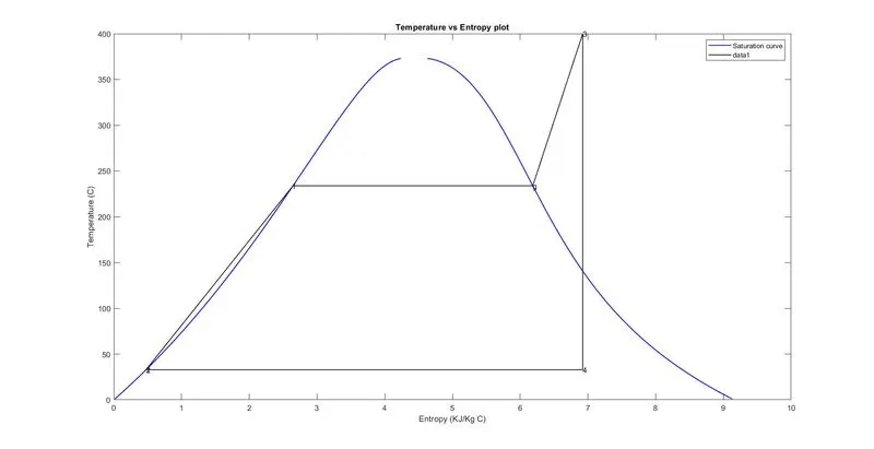
Resulted Plots
After providing following inputs in command window
Turbine Inlet temperature = 400° C
Turbine Inlet Pressure = 30 bars
Turbine Outlet Pressure = 0.05 bars = Condenser Inlet Pressure
we will get :-
1. Plot 1 :- Plot of Temperature vs Entropy
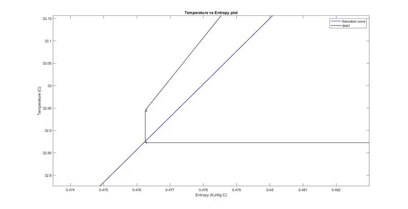
1. Plot 1 :- Plot of Enthalpy vs Entropy
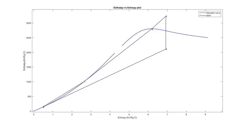
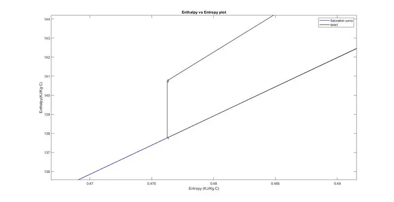
Results:-
- Net work output = 1.1179e+03
- Back work ratio (%)= 0.2674