Week 4.1 - Genetic Algorithm

GENETIC ALGORITHM IN MATLAB

AIM

1) To write a code in MATLAB to optimise the stalagmite function and find the global maxima of the function.

2) To understand more about genetic algorithm and to determine how it works

INTRODUCTION

GENETIC ALGORITHM

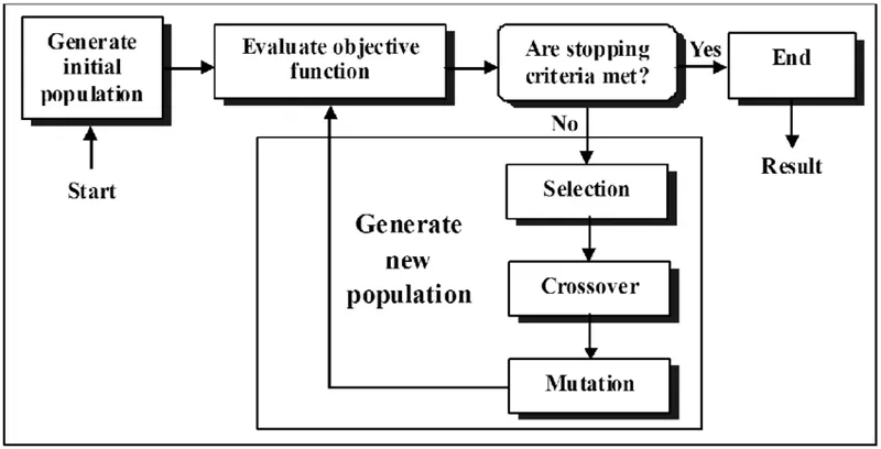
The genetic algorithm is an algorithm used for solving both constrained and unconstrained optimisation problems. A genetic -

algorithm is a search heuristic that is inspired by charles Darwin's theory of natural evolution.Genetic algorithm starts with an initial

set of random solutions called population. each individual in the population is called a chromosome representing a solution to the

problem at hand . The chromosomes evolve through successive iterations , called generations . During each generation ,the chromos-

ome are evolved using some measure of fitness . fitter chromosomes have higher probabilities of being selected . After several genera-

tions , the algorithm converge to the best chromosome , which hopefully represents the optimum or sub-optimal solution to the problem.

Syntax of ga

1)x=ga(fun,nvars)

fun=function name or function handle

nvars=no: of variables

2)x=ga(fun,nvars,A,b)

A=linear inequality constraints ,as real matrix

b=linear inequality constrains , as real vector

3)x=ga(fun,nvars,A,b,Aeq,beq)

Aeq,beq = linear equalities of A and b

4)x=ga(fun,nvars,A,b,Aeq,beq,lb,ub)

lb=lower bound

ub=upper bound

5)x=ga(fun,nvars,A,b,Aeq,beq,lb,ub,nonlcon)

nonlcon=non linear constrains specified as a function handle or a function name

6)x=ga(fun,nvars,A,b,Aeq,beq,lb,ub,nonlcon,options)

options=optimisation options,specified as output optimisation

• STEP BY STEP EXPLANATION

First, we write a code to define the stalagmite function . Here we break down the formula in to 4 terms for convenience.

Then we write main code were we define two inputs x and y both of which are one dimensional equally spaced array -

containing 150 elements . We utilise meshgrid command to create an array of x and y values .

Now we use for loop to input values of 2D array in stalagmite function.Here we encounter an problem , ie, every time

the code executed diffrent values of stalagmite function are obtained.This is overcomed by introducing another loop in

to the code .Then we input these values in genetic algorithm ,ga function is used for this.

To improve the genetic algorithm , we undertakes 3 studys to optimise the function so that we can accuratly find the -

global maxima of the function. negative sign given to the functional term in order to get the maxima value,ga generally

provide the minima value instead.

In 1st case we evaluate all possible global maxima for all the iterations using a loop.We plot two in one figure using sub-

plot in one figure using subplot command .'surfc' command is used for x v/s y graph and for function max v/s iteration

we use simple 'plot' command . The values in figure(1) are unbounded values.

In 2nd case we put an upper bound and lower bound on 'ga' function and again plot two plots as same as the first plot.

In 3rd case , we increase the ga iterations . in ga , after successive iterations ,the population evolves toward an optimal

solution .ie,more the number of iterations ,more optional the solution will be. Now we use same commands to plot the

graph and the curve

FUNCTION CODE

function [f]= stalagmite_fun(inputs)
x=inputs(1);
y=inputs(2);


term1= (sin((5.1*pi*x)+0.5)).^6;
term2= (sin((5.1*pi*y)+0.5)).^6;

term3=exp((-4)*log(2)*((x-0.0667).^2)/0.64);
term4=exp((-4)*log(2)*((y-0.0667).^2)/0.64);


f=-(term1*term2*term3*term4);

MAIN CODE

clear all
close all
clc

% defining search space
x=linspace(0,0.6,150);
y=linspace(0,0.6,150);


%creating 2d mesh
[xx,yy]=meshgrid(x,y);

for i=1:length(xx)
    for j=1:length(yy)
        inputs(1)=xx(i,j);
        inputs(2)=yy(i,j);
        F(i,j)=stalagmite_fun(inputs);

    end
end
 surfc(x,y,F)
% STUDY-1 Statistical behaviour of ga
num_cases=50;
tic
for i=1:num_cases
    [inputs,fopt(i)]=ga(@stalagmite_fun,2);
    xopt(i)=inputs(1);
    yopt(i)=inputs(2);
end


study1_time=toc;
figure(1)
subplot(2,1,1)
hold on
surfc(xx,yy,-F)
shading interp
plot3(xopt,yopt,-fopt,'marker','o','MarkerSize',5,'MarkerFaceColor','r')
title('unbounded inputs')
subplot(2,1,2)
plot(-fopt)
xlabel('iterations')
ylabel('functions maxima')

% statistical behaviour with upper bound and lower bound
tic

for i=1:num_cases
    [inputs,fopt(i)]=ga(@stalagmite_fun,2,[],[],[],[],[0;0],[0.3;0.3],[],[]);
    xopt(i)=inputs(1);
    yopt(i)=inputs(2);
end
study2_time=toc;
figure(2)
subplot(2,1,1)
hold on
surfc(xx,yy,-F)
shading interp
plot3(xopt,yopt,-fopt,'marker','o','MarkerSize',5,'MarkerFaceColor','r')
title('bounded inputs')
subplot(2,1,2)
plot(-fopt)
xlabel('iterations')
ylabel('functions maxima')

%CASE3 INCREASING NO OF ITERATIONS
tic
options=optimoptions('ga');
options=optimoptions(options,'PopulationSize',500);
for i=1:num_cases
    [inputs,fopt(i)]=ga(@stalagmite_fun,2,[],[],[],[],[0;0],[0.3;0.3],[],options);
    xopt(i)=inputs(1);
    yopt(i)=inputs(2);
end
study3_time=toc;
figure(3)
subplot(2,1,1)
hold on
surfc(x,y,-F)
shading interp
plot3(xopt,yopt,-fopt,'marker','o','MarkerSize',5,'MarkerFaceColor','b')
title('bounded inputs with increased population size')
subplot(2,1,2)
plot(-fopt)
xlabel('iterations')
ylabel('functions maxima')

CONCLUSION

Explained the concept of genetic algorithm and explained the syntax of ga in MATLAB.