Genetic Algorithm
AIM
To write a code in MATLAB to optimise the stalagmite function and find the global maxima of the function
OBJECTIVE
- Code for optimise the stalagmite function
- Find Global Maxima in the function
- Explain genetic alogorithms and syntax for ga
- Plot graphs for all three studies and for function maximum vs no. of iterations
STALAGMITE
A stalagmite is a type of rock formation that rises from the floor of a cave due to the accumulation of material deposited on the floor from ceiling drippings. In here stalagmite has represents the program's output shape
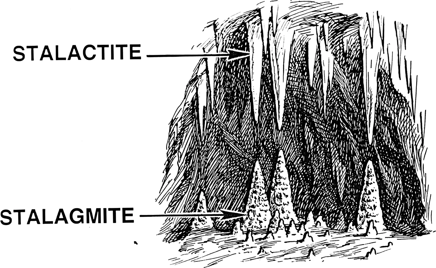
GENETIC ALGORITHM(Inspired by Charles Darwin)
- Genetic algorithms came from the research of John Holland, in the University of Michigan, in 1960 but won't become popular until the 90's and it's a popular "Metaheuristic"
- It's based on the mechanism of natural selection in "Charles Darwin's Theory" of natural evolution
- Their main purpose is to be used to solve problems where deterministic algorithms are too costly.
- It's one of the "Machine Learning" algorithms that is used to optimise results and it's used in business, scientific & engineering circles
- In the industry, genetic algorithms are used when traditional ways are not efficient enough
- A genetic algorithm (GA) is a method for solving problems that are not well suited for standard optimization algorithms
- The algorithm repeatedly modifies a population of individual solutions
- At each step, the genetic algorithm randomly selects individuals from the current population and uses them as parents to produce the children for the next generation
- Over successive generations, the population "evolves" toward an optimal solution
METAHEURISTIC DEFINITION
In computer science and mathematical optimization, a metaheuristic is a higher-level procedure or heuristic designed to find, generate, or select a heuristic that may provide a sufficiently good solution to an optimization problem, especially with incomplete or imperfect information or limited computation capacity
5 General parameters were used in GA:
- Initial Population
- Fitness Function
- Selection
- Crossover
- Mutation
Initial Population
This step starts with guessing of initial sets of values which may or may not include the optimal values. These sets of values are called as ‘chromosomes’ and the step is called "initialize population"
Fitness Function
In this step, the value of the objective function for each chromosome is computed. The value of the objective function is also called "fitness value"
Selection
This step is very important and is called "selection" because fittest chromosomes are selected from the population for subsequent operations
Crossover
In this step, chromosomes are expressed in terms of genes. This can be done by converting the values into binary strings. This step is called "crossover"
Mutation
Mutation is the process of altering the value of gene
FLOW CHART
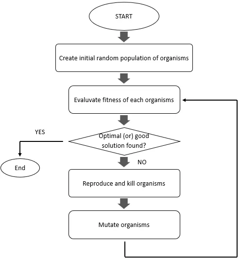
MATHEMATICAL EQUATION
To find global maxima:
`f=(f1x.f2x.f1y.f2y)`
To find global minima:
`f=-(f1x.f2x.f1y.f2y)`
where,
`f1x=[sin(5.1pix+0.5)]^6`
`f2x=exp[-4ln(2)(x-0.0667)^2/0.64]`
`f1y=[sin(5.1piy+0.5)]^6`
`f2y=exp[-4ln(2)(y-0.0667)^2/0.64]`
PROGRAM
1. Main Program(Optimise the stalagmite function by genetic algorithm)
clear all
close all
clc

%Defining search space
x = linspace(0,0.6,150);
y = linspace(0,0.6,150);

%Creating 2D mesh
[xx,yy] = meshgrid(x,y);

%Evaluvating Stalagmite function
 for i = 1:length(xx)
    for j = 1:length(yy)
        input_vector(1) = xx(i,j);
        input_vector(2) = yy(i,j);
        f(i,j) = stalagmite(input_vector);
    end
 end

%Plotting
surfc(xx,yy,f)
shading interp
[inputs,fval] = ga(@stalagmite,2);
xlabel('x value')
ylabel('y value')
2. Stalagmite Function Call Program(Global Maxima)
function [f] = stalagmite(input_vector)

x = input_vector(1);
y = input_vector(2);

f1x = (sin(5.1*pi*x+0.5))^6;
f2x = (sin(5.1*pi*y+0.5))^6;

f1y = exp(-4*log(2)*((x-0.0667)^2/0.64));
f2y = exp(-4*log(2)*((y-0.0667)^2/0.64));

f = (f1x*f2x*f1y*f2y);

end
3. Main Program(Optimise the stalagmite function by genetic algorithm)
clear all
close all
clc

%defining search space
x = linspace(0,0.6,150);
y = linspace(0,0.6,150);

[xx,yy] = meshgrid(x,y);
num_cases = 50;

%Evaluvating stalagmite finction
for i = 1:length(xx)
    for j = 1:length(yy)
        input_vector(1) = xx(i,j);
        input_vector(2) = yy(i,j);
        f(i,j) = stalagmite(input_vector);
    end
end

tic
%Study1 - Statistic Behavior
for i = 1:num_cases
    [inputs,fopt(i)] = ga(@stalagmite,2);
    xopt(i) = inputs(1);
    yopt(i) = inputs(2);
end
Study1_time = toc;

%Plotting
figure(1)
subplot(2,1,1)
hold on
surfc(x,y,f)
plot3(xopt,yopt,fopt,'marker','o','markersize',5,'markerfacecolor','r')
shading interp
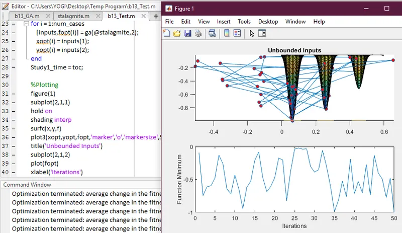
title('Unbounded Inputs')
subplot(2,1,2)
plot(fopt)
xlabel('Iterations')
ylabel('Function Minimum')

tic
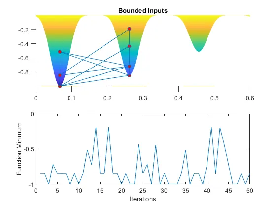
%Study2 - Statistic Behavior with upper & lower bounds
for i = 1:num_cases
    [inputs,fopt(i)] = ga(@stalagmite,2,[],[],[],[],[0:0],[0.6:0.6]);
    xopt(i) = inputs(1);
    yopt(i) = inputs(2);
end
Study2_time = toc;

%Plotting
figure(2)
subplot(2,1,1)
hold on
surfc(x,y,f)
plot3(xopt,yopt,fopt,'marker','o','markersize',5,'markerfacecolor','r')
shading interp
title('Bounded Inputs')
subplot(2,1,2)
plot(fopt)
xlabel('Iterations')
ylabel('Function Minimum')

tic
%Study3 - Increasing with ga Iterations
options = optimoptions('ga');
options = optimoptions(options,'populationsize',1500);

for i = 1:num_cases
    [inputs,fopt(i)] = ga(@stalagmite,2,[],[],[],[],[0:0],[0.1:0.1],[],[],options);
    xopt(i) = inputs(1);
    yopt(i) = inputs(2);
end
Study3_time = toc;

%Plotting
figure(3)
subplot(2,1,1)
hold on
surfc(x,y,f)
plot3(xopt,yopt,fopt,'marker','o','markersize',5,'markerfacecolor','r')
shading interp
title('Bounded Inputs with Population Size')
subplot(2,1,2)
plot(fopt)
xlabel('Iterations')
ylabel('Function Minimum')
4. Stalagmite Function Call Program(Global Minima)
function [f] = stalagmite(input_vector)

x = input_vector(1);
y = input_vector(2);

f1x = (sin(5.1*pi*x+0.5))^6;
f2x = (sin(5.1*pi*y+0.5))^6;

f1y = exp(-4*log(2)*((x-0.0667)^2/0.64));
f2y = exp(-4*log(2)*((y-0.0667)^2/0.64));

f = -(f1x*f2x*f1y*f2y);

end
CODE EXPLAINATION
- First of all, we have to program the stalagmite sub-functions for global maxima and global minima by the appropriate mathematical formulae has given
- Now program the main function to find the global maxima, by using the commands of linspace(to define the search space), meshgrid(to create 2 dimensional mesh) and nested-for loop(to evaluvate the stalagmite function)
- Then call the sub function(stalagmite) in the nested-for loop command
- Then plot the output with surfc(to creates a 3 dimensional surface plot with a contour plot underneath), shading interp(to controls the color shading of surface), plot3(to plot a set of coordinates connected by line segments)
- By using these above commands will shows the output of global maxima by the initial inputs
- Now we going to find the global minima by optimise the random inputs
- In this optimisation, we going follows the 3 parametes which are selection, crossover and mutation
- By following these parameters we going to seperate the codes into 3 studies to know the statistical behaviors of it
- Here the global minima's stalagmite call function has used on the entire code
- And we going to follow the same code procedure as what we did before in the global maxima program with the small modifications in "ga" solver commands where inside the each study cases(appropriate parameters) of for-loop command
PLOT OUTPUTS
1. For Global Maxima
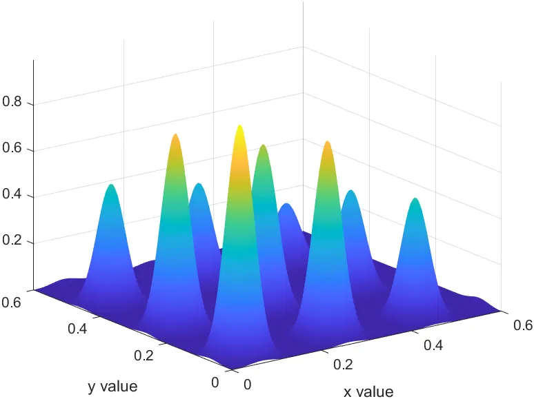
2. For Global Minima(Finding Minimum Function)
I. Study1 - Statistical Behavior
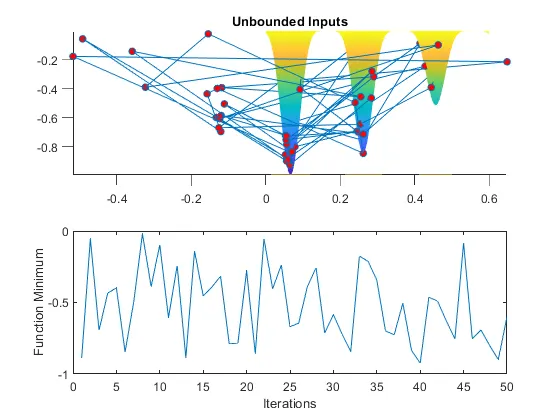
II. Study 2 - Statistical Behavior with Upper & Lower bounds
III. Study 3 - Increasing GA iterations
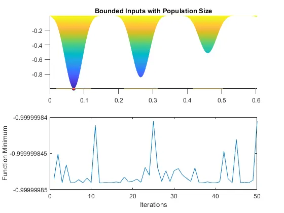
Note: From the 3rd plot we got the single point, by increasing the population size
ERROR OCCURED
1. Got an surface color issue, even I have used the command("shading interp")...line 34
Solution: Re-command it after the plot3 command
REFERENCES
1. Genetic Algorithm with Solved Example(Selection,Crossover,Mutation)