Curve Fitting
AIM
To write code to fit a linear and cubic polynomial for the Cp data
OBJECTIVE
- Write the curve fitting program with original data by using polynomials
- Plot the linear and cubic fit curves along with the raw data points
CURVE FITTING
Curve fitting is the process of constructing a curve, or mathematical function, that has the best fit to a series of data points, possibly subject to constraints. Curve fitting can involve either interpolation, where an exact fit to the data is required, or smoothing, in which a "smooth" function is constructed that approximately fits the data
FITTING LINES AND POLYNOMIAL FUNCTIONS TO DATA POINTS
Most commonly, one fits a function of the form y=f(x)
- The first degree polynomial equation
y=ax+b - is a line with slope a. A line will connect any two points, so a first degree polynomial equation is an exact fit through any two points with distinct x coordinates.
- If the order of the equation is increased to a second degree polynomial, the following results:
y=ax^2+bx+c - This will exactly fit a simple curve to three points
- If the order of the equation is increased to a third degree polynomial, the following is obtained:
y=ax^3+bx^2+cx+d - This will exactly fit four points
- If the order of the equation is increased to a fourth degree polynomial, the following is obtained:
y=ax^3y+bxy^2+cx^2+dx+e - This also exactly fit five points
GOODNESS OF FIT (OR) GOODNESS OF PREDICTION
After using graphical methods to evaluate the goodness of fit, you should examine the goodness-of-fit statistics Curve Fitting Toolbox software supports these goodness-of-fit statistics for parametric models:
- The sum of squares due to error (SSE)
- R-square
- Adjusted R-square
- Root mean squared error (RMSE)
For the current fit, these statistics are displayed in the Results pane in the Curve Fitting app. For all fits in the current curve-fitting session, you can compare the goodness-of-fit statistics in the Table of fits
1. Sum of Squares Due to Error (SSE)
This statistic measures the total deviation of the response values from the fit to the response values. It is also called the summed square of residuals and is usually labeled as SSE
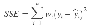
A value closer to 0 indicates that the model has a smaller random error component, and that the fit will be more useful for prediction
2. R-Square
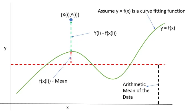
- This statistic measures how successful the fit is in explaining the variation of the data. Put another way, R-square is the square of the correlation between the response values and the predicted response values
- It is also called the square of the multiple correlation coefficient and the coefficient of multiple determination
- R-square is defined as the ratio of the sum of squares of the regression (SSR) and the total sum of squares (SST)
SSR is defined as
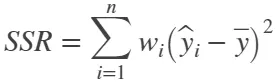
SST is also called the sum of squares about the mean, and is defined as
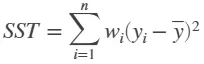
where SST = SSR + SSE. Given these definitions, R-square is expressed as
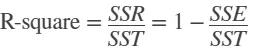
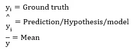
where,
3. Degrees of Freedom Adjusted R-Square
- This statistic uses the R-square statistic defined above, and adjusts it based on the residual degrees of freedom. The residual degrees of freedom is defined as the number of response values n minus the number of fitted coefficients m estimated from the response values
v = n-m
- v indicates the number of independent pieces of information involving the n data points that are required to calculate the sum of squares
- The adjusted R-square statistic is generally the best indicator of the fit quality when you compare two models that are nested — that is, a series of models each of which adds additional coefficients to the previous model

- The adjusted R-square statistic can take on any value less than or equal to 1, with a value closer to 1 indicating a better fit. Negative values can occur when the model contains terms that do not help to predict the response
4. Root Mean Squared Error
- This statistic is also known as the fit standard error and the standard error of the regression. It is an estimate of the standard deviation of the random component in the data, and is defined as

- where MSE is the mean square error or the residual mean square

- Just as with SSE, an MSE value closer to 0 indicates a fit that is more useful for prediction
Using this four qualities matlab effectively deduces the goodness of fit, typically is R square is greater than 0.95 the fit is assumed to be good
MODEL GRAPH
CODE SAMPLE
1. Linear Fit
%linear Fit

clear all
close all
clc

%preparing the data
cp_data = load('data');
temperature = cp_data(:,1);    %1st column Temperature data
cp = cp_data(:,2);             %2nd column cp data

%curve fit
co_effs = polyfit(temperature,cp,1)       %cp = ax+b(1polynamial;Linear)
pred_cp = polyval(co_effs,temperature);   %polynomial value

%compare curve fit with original data

plot(temperature,cp,'linewidth',3)        %plotting with original data
hold on
plot(temperature,pred_cp,'linewidth',3)   %plotting with predicted data
xlabel('Temperature [K]');
ylabel('Specific Heat [KJ/Kmol-K]')
title('Linear Fit Curve')
legend('Original Data','Curve Fit')
grid on
2. Cubic Fit
%Cubic Fit

clear all
close all
clc

%preparing the data
cp_data = load('data');
temperature = cp_data(:,1);     %1st column Temperature data
cp = cp_data(:,2);              %2nd column cp data

%curve fit
co_effs = polyfit(temperature,cp,3)       %cp = ax^3+bx^2+cx+d(3polynamials;Cubic)
pred_cp = polyval(co_effs,temperature);   %polynomial value

%compare curve fit with original data

plot(temperature,cp,'linewidth',3)        %plotting with original data
hold on
plot(temperature,pred_cp,'linewidth',3)   %plotting with predicted data
xlabel('Temperature [K]');
ylabel('Specific Heat [KJ/Kmol-K]')
title('Cubic Fit Curve')
legend('Original Data','Curve Fit Data')
grid on
CODE SAMPLE EXPLAINATION
- First of all, type clear all, close all, clc from the beginning
- Then use the load command to prepare the original data file, call it as 'cp_data' and take out the temperature, specific heat(cp) value and assign as seperately
- Now we going to perform a curve fit with the help of two commands, they are
i. polyfit (Polynomial Fit)
polyfit(x,y,n) finds the coefficients of a polynomial p(x) of degree n that fits the y data by minimizing the sum of the squares of the deviations of the data from the model (least-squares fit)
ii. polyval (Polynomial Value)
polyval(p,x) returns the value of a polynomial of degree n that was determined by polyfit, evaluated at x
- Now compare the both data to find out the googness of prediction by using plot command
- Provide x and y labels, title, legend for each curve and turn ON the grid
- Similar program for both linear and cubic, just change the 'n' value in "polyfit" for each time
PLOT DIAGRAM
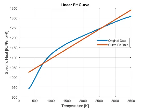
1.Linear Fit
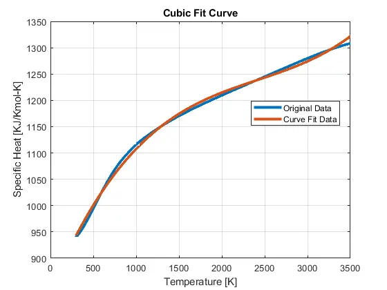
2.Cubic Fit
Solution:
By comparing this above two curves, Cubic fit's predicted curve is closely travels along with the original curve
CURVE FITTING TOOL-BOX
- Curve Fitting Toolbox provides an app and functions for fitting curves and surfaces to data. The toolbox lets you perform exploratory data analysis, preprocess and post-process data, compare candidate models, and remove outliers. You can conduct regression analysis using the library of linear and nonlinear models provided or specify your own custom equations
- The library provides optimized solver parameters and starting conditions to improve the quality of your fits. The toolbox also supports nonparametric modeling techniques, such as splines, interpolation, and smoothing
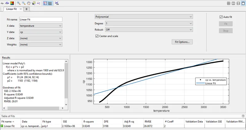
1.Linear Fit
2.Cubic Fit
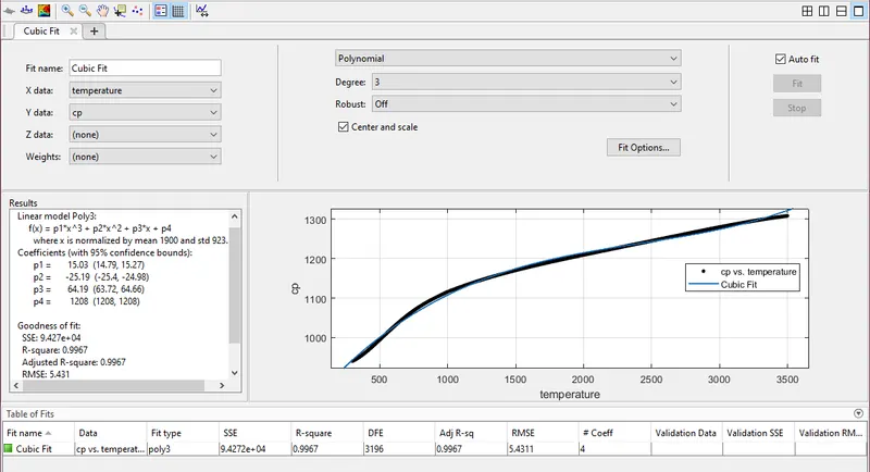
Note: By using the curve fit tool box, Compare the above two results,
Linear fit: R^2 = 0.9249
Cubic Fit: R^2 = 0.9967
Here, cubic fit's R square value is close to 1, so it's the "goodness of fit"
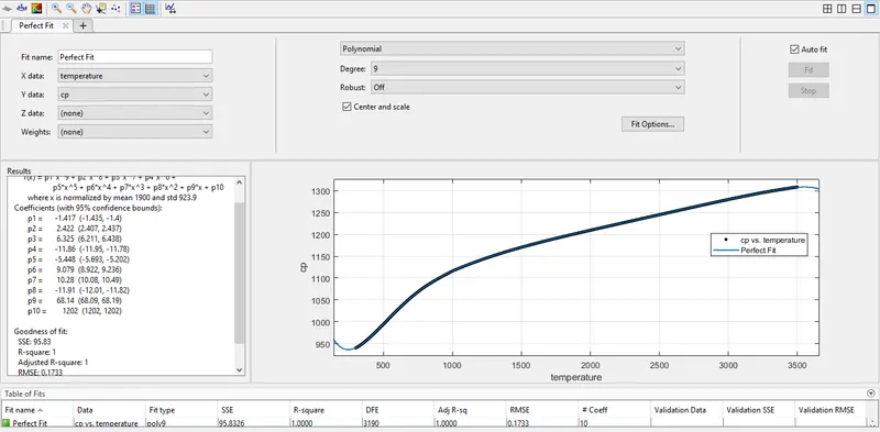
NOTE: We can also use the curve fitting tool box to minimize the error by increasing the degree of polynomials, From the evaluation we can get R Square value as 1 in both 8 & 9 degree, but here I choosen the best fit in 9 degree
SPLITWISE METHOD
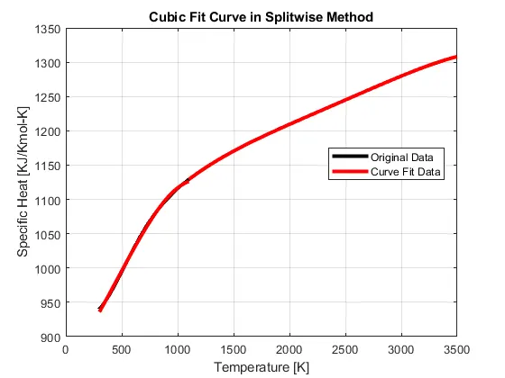
To improve the result of cubic fit curve, we have to split the data in 4 sub-parts by using splitwise method before that we need to load the original data
PROGRAM
%Cubic Fit(Splitwise Method)

clear all
close all
clc

%preparing the data
cp_data = load('data');
temperature = cp_data(:,1);     %1st column Temperature data
cp = cp_data(:,2);              %2nd column cp data

%splitting data
temperature1 = cp_data(1:800,1);
cp1 = cp_data(1:800,2);

temperature2 = cp_data(801:1600,1);
cp2 = cp_data(801:1600,2);

temperature3 = cp_data(1601:2400,1);
cp3 = cp_data(1601:2400,2);

temperature4 = cp_data(2401:3200,1);
cp4 = cp_data(2401:3200,2);

%curve fit: cubic (3rd degree polynomials)
co_effs1 = polyfit(temperature1,cp1,3);
pred_cp1 = polyval(co_effs1,temperature1);

co_effs2 = polyfit(temperature2,cp2,3);
pred_cp2 = polyval(co_effs2,temperature2);

co_effs3 = polyfit(temperature3,cp3,3);
pred_cp3 = polyval(co_effs3,temperature3);

co_effs4 = polyfit(temperature4,cp4,3);
pred_cp4 = polyval(co_effs4,temperature4);

%compare curve fit with original data
plot(temperature,cp,'linewidth',3,'color','k')
hold on
plot(temperature1,pred_cp1,'linewidth',3,'color','r');
plot(temperature2,pred_cp2,'linewidth',3,'color','r');
plot(temperature3,pred_cp3,'linewidth',3,'color','r');
plot(temperature4,pred_cp4,'linewidth',3,'color','r');
xlabel('Temperature [K]')
ylabel('Specific Heat [KJ/Kmol-K]')
title('Cubic Fit Curve in Splitwise Method')
legend('Original Data','Curve Fit Data')
grid on

%Calc the error
pred_cp = [pred_cp1;pred_cp2;pred_cp3;pred_cp4];
error = cp-pred_cp;
fprintf('Maximum Error is');
disp(max(error));
NOTE: The least error in this case will be 4.3944, the plot shows the reference as below,
PLOT DIAGRAM
QUESTIONS:
How to make a curve fit perfectly?
The most common way to fit curves to the data by using linear regression and increasing x points by the degree of polynomials, which means the curve travels through the every points
How to get the best fit?
It's the straight line drawn through the maximum number of points on a scatter plot on balancing an equal number of points on above and below the line
What could be done to improve the cubic fit?
It's by using "splitwise method", this method turns the load data into 4 sub-parts of data. It helps to minimize the error than the other ways
ERRORS DURING PROGRAMMING
No more errors occur this time
REFERENCES