Solving second order ODEs

AIM

To write a program in Matlab that will simulate the simple pendulum motion

OBJECTIVE

• Write the program to simulate the transient behavior of a simple pendulum
• Animate a simple pendulum by the program using Matlab

ORDINARY DIFFERENTIAL EQUATION

An ordinary differential equation (ODE), in Mathematics, is an equation which consists of one or more functions of one independent variable along with their derivatives. A differential equation is an equation that contains a function with one or more derivatives. But in the case ODE, the word ordinary is used for derivative of the functions for the single independent variable.

In case of other types of differential equations, it is possible to have derivatives for functions more than one variable. The types of DEs are partial differential equation, linear and non-linear differential equations, homogeneous and non-homogeneous differential equation.

SIMPLE PENDULUM

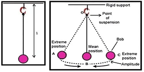
• A simple pendulum is a mechanical arrangement that demonstrates periodic motion. A point mass attached to a light inextensible string and suspended from fixed support is called a simple pendulum.
• The vertical line passing through the fixed support is the mean position of a simple pendulum.
• The vertical distance between the point of suspension and the centre of mass of the suspended body (when it is in mean position) is called the length of the simple pendulum denoted by L.

ODE DERIVATION

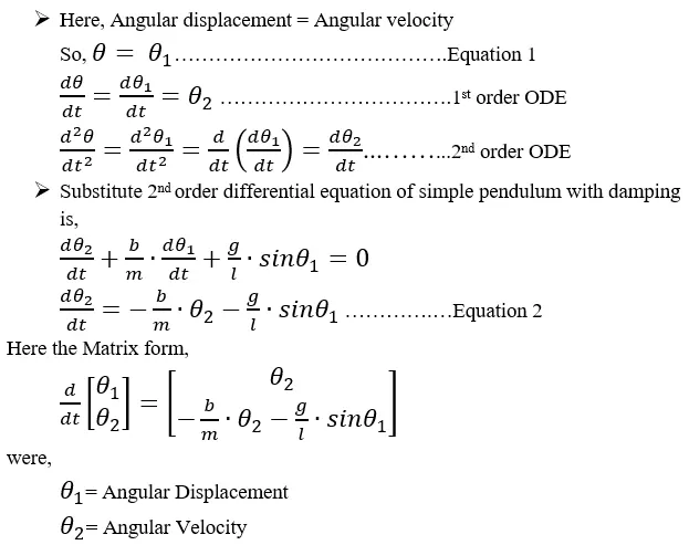
• Now, we going to apply the above equation in Matlab to find out the 'Angular dispacement' and 'Angular Velocity' with respect to time

CODE SAMPLE

1. ODE Function Call Program

function [dtheta_dt] = ode_func(t,theta,b,m,g,l)

   theta1 = theta(1);
   theta2 = theta(2);

   dtheta1_dt = theta2;
   dtheta2_dt = -(b/m)*theta2-(g/l)*sin(theta1);

   dtheta_dt = [dtheta1_dt;dtheta2_dt];

end

2. Main Program(Single Pendulum Animation using ODE by calling function)

Given Inputs:

L=1 metre, m=1 kg, b=0.05. g=9.81 m/s2. Simulate the motion between 0-20 sec, for angular displacement=0,angular velocity=3 rad/sec at time t=0.

clear all
close all
clc

%inputs
   b = 0.05; %(damping coefficient)
   m = 1; %(mass of ball in kg)
   g = 9.81; %(gravity in m/s^2)
   l = 1; %(length of the pendulum in metre)

%initial condition
   t_span = linspace(0,20,400);

   theta_0 = [0;3];

%Evaluvate ODE
   [t,result] = ode45(@(t,theta) ode_func(t,theta,b,m,g,l),t_span,theta_0);

%Plotting angular displacement and angular velocity
   figure(1)
   plot(t,result(:,1),'linewidth',2)
   hold on
   plot(t,result(:,2),'linewidth',2)
   hold off
   axis([0 20 -5 5])
   xlabel('Time(sec)')
   ylabel('Angular Displacement(rad) & Angular Velocity(rad/s)')
   grid on
   title('Single Pendulum Using ODE')
   legend('Angular Displacement','Angular Velocity')

ct = 1;
for i = 1:length(t_span)
   THETA(i) = result(i,1);
   x0 = 0;
   y0 = 0;
   
   x1 = l*sin(THETA(i));
   y1 = -l*cos(THETA(i));
   
%Plotting single pendulum motion
   figure(2)    %motion is plotted
   plot([x0 x1],[y0 y1],'color','c','linewidth',3) %plotting string as a line
   hold on
   plot(x1,y1,'marker','o','markersize',25,'markerfacecolor','g','markeredgecolor','k') %plotting the bob
   hold off
   line([-1 1],[0 0],'color','r','linewidth',3) %plotting the roof
   axis([-1.5 1.5 -1.5 0.5])
   grid on
   title('Motion of Single Pendulum')
   pause(0.05)
   M(ct) = getframe(gcf);
ct = ct+1; 
end

%Animate Single Pendulun
   movie(M)
   videofile = VideoWriter('Simple Pendulum using ODE.avi','Uncompressed AVI');
   open(videofile)
   writeVideo(videofile,M)
   close(videofile)

CODE SAMPLE E4XPLAINATION

• First we have to starts with clear all,close all, clc
• Take down the given inputs as initial values and the inital condition is angular displacement(θ1=0rad or deg) angular velocity(θ2=3rad/sec) were entered in theta_0
• The total time span is 20 seconds with 400 time intervals which used the linspace command weree entered in t_span
• Here the calling function is used to call the user-defined function of 'ode_func' where mentioned in the above code sample section
• The first code sample(ode function call program) is programmed by the derivation of 2nd order ODE
• Now all the corresponding values are entered into the 2nd order ODE evaluvation by using 'ode 45' syntax
• ODE 45 - Solve nonstiff differential equations — medium order method, where ode45 is a versatile ODE solver and is the first solver you should try for most problems. However, if the problem is stiff or requires high accuracy, then there are other ODE solvers that might be better suited to the problem
• This which provides the outputs to [t,result]-LHS as for each time intervals
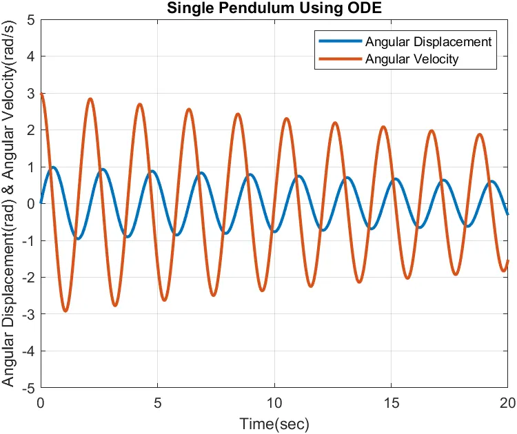
• Then plot by angular displacement and angular velocity with respect to time
• Use figure(1) command for seperate output, after that plot the angular displacement first as "plot(t,result(:,1)", then use the 'hold on' and plot angular velocity as "plot(t,result(:,2)", then use the 'hold off' for a proper output
• Then provide a proper axis, label names,legend and title to the plot
• Now use the for-loop command for plotting the transient behavior of a simple pendulum
• 'i' value has called into THETA(i) like,

i = 1:length(t_span)

THETA(i) = result(i,1);

• The calculate the coordinates of string x0,y0 and x1,y1. Initially I have taken x0 = 0, y0 = 0, then calculated x1 and y1 as

x1 = l*sin(THETA(i));

y1 = -l*cos(THETA(i));

• Now we going to simulate the simple pendulum by plotting, use figure(1) command for seperate output, here plot the string like a line with the coordinates of [x0 x1],[y0 y1],[x1 x2],[y1 y2] and make the linewidth with enough values
• Plot the pendulum bob by using the commands of 'marker','markersize','markerfacecolor','markeredgecolor' with a enough shape and markersize
• And also plot a line with enough values which seems like a roof on top in the animation
• Then give an axis (-x x -y y) as a boundary,title,etc.,
• Use the pause command to pause the execution for n number of seconds before continuing, where n can be any real number
• After that, use getframe command to capture the figure as movie frame and call it in M(ct)
• In getframe, we dealing with (gcf) like getframe(gcf), to return the current figure handle
• And we use (ct - counter) before in the beginning and ending of the for-loop for an increment, like ct = 1; and ct = ct+1;
• After the For-loop completes, use the movie command to plays the movie frames in array M once
• Create a videofile by the command of VideoWriter with a appropriate filename and format
• Finally, use the writeVideo command to writes data from an array to the video file

PLOT DIAGRAM

VIDEO LINK

https://youtu.be/3ZSSyQoErRA/

ERRORS DURING PROGRAMMING

1. Manual error: Figure(2) animation goes wrong

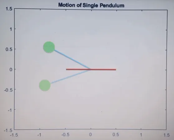
Reason: Before the animation, the pendulum needs an initial coordinates values of (x0 x1),(y0 y1),so we need to provide a right calculation, so here is I gave a wrong x1 and y1 calculation.

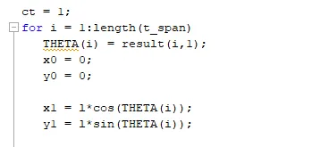
Solution: After that I made a correction in that, actual calculation of x1 and y1 is,

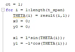
We need to plot in 3rd and 4th quadrant, Refer the quadrant graph of trignometry,

2. Manual error: plot displayed only angular displacement

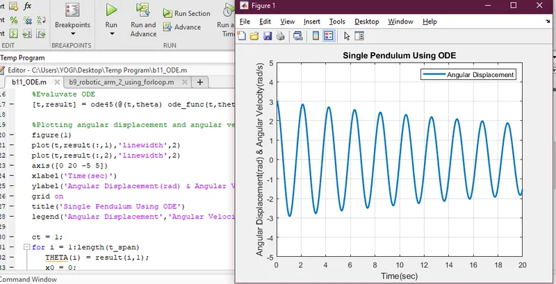
Solution: I has forget to put "hold on" and "hold off" commands on next to line 21 and 22