Week 4.1 - Genetic Algorithm

1) CODE -

%Program to find global maxima of function
clear all; close all; clc
x = linspace(0,0.6,150); % x Search space
y= linspace(0,0.6,150);% y search space
num_cases = 50 %50 times for function will run
[xx yy] = meshgrid(x,y);
for i = 1:length(xx)
    for j = 1:length(yy)
        input_vector(1)=xx(i,j)
        input_vector(2)=yy(i,j)
        
f(i,j) = stalagmite_func(input_vector);
    end
end

%Study 1 - Statistical Behaviour 
for i = 1:num_cases
    [inputs,fval(i)] = ga(@stalagmite_func,2);
    xopt(i) = inputs(1);
    yopt(i) = inputs(2);
    
end
figure(1)
subplot(2,1,1)
surf(x,y,-f) %Adding minus sign to get positive value
shading interp %Remove grid lines and makes smooth curve
hold on
plot3(xopt,yopt,-fval,'Marker','o','MarkerSize',5,'markerfacecolor','r'); %3d Plot
title('Unbounded Inputs');
subplot(2,1,2);
plot(-fval);%Adding minus sign to get positive value
xlabel('Iteration');
ylabel('Function Minimum');

%Study 2 - Statistical Behaviour with upper & Lower bounds
for i = 1:num_cases
    [inputs fval(i)]=ga(@stalagmite_func,2,[],[],[],[],[0;0],[0.4;0.4]);
    xopt(i)=inputs(1);
    yopt(i)=inputs(2);
end

figure(2)
subplot(2,1,1)
surf(x,y,-f)%Adding minus sign to get positive value
shading interp
hold on
plot3(xopt,yopt,-fval,'Marker','o','MarkerSize',5,'markerfacecolor','r');
title('Bounded Inputs');
subplot(2,1,2);
plot(-fval);%Adding minus sign to get positive value
xlabel('Iteration');
ylabel('Function F maximum');

%Study 3 - Increasing GA Iterations
options = optimoptions('ga');
options = optimoptions(options,'PopulationSize',250);

for i = 1:num_cases
    [inputs fval(i)]=ga(@stalagmite_func,2,[],[],[],[],[0;0],[0.4;0.4],[],[],options);
    xopt(i)=inputs(1);
    yopt(i)=inputs(2);
end

figure(3)
subplot(2,1,1)
surf(x,y,-f) %Adding minus sign to get positive value
shading interp
hold on
plot3(xopt,yopt,-fval,'Marker','o','MarkerSize',5,'markerfacecolor','r');
title('Bounded Inputs with increased population');
subplot(2,1,2);
plot(-fval); %Adding minus sign to get positive value
xlabel('Iteration');
ylabel('F maximum');

Explanation -

First of all, define the search space for the ga solver with the help of linspace command and then convert it to a 2D dimensional mesh.

num_cases will tell the function how many numbers of times for function will run.

Then we evaluate the stalagmite function with 2 input vectors x and y which corresponds to fvalue which is in the z-direction.

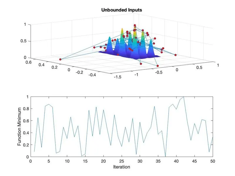
In study 1 - we saw statistical behaviour of points in the graph in which we called stalagmite function with 2 variables without any boundaries.

The first figure shows lots of points in the graph area and also in subplot points are changing their value at every iteration hence results are inaccurate.

plot3 is the 3d line plot command.

In study 2 - We apply boundaries to the GA solver equation in between 0 to 0.4 with linear equality and inequality constraints.

Hence we get fewer fvalues in between 0 & 0.4 but still, it is not optimised.

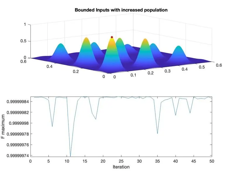
In study 3 - We used the optimisation option command with GA solver and increases its iteration range from 150 to 250.

Which gives a more accurate graph and single maximum value.

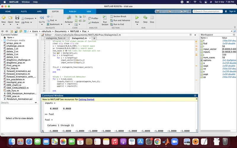
GLOBAL MAXIMA (fval) IS -1.0000 at x=0.0668 & y=0.0668

2)GA(Genetic Algorithm) -

The genetic Algorithm in MATLAB is used to find the minimum value from a function. It is an inbuild solver which gives us an optimised value of any problem which is used to find optimal or near-optimal solutions.

3)SCREENSHOTS -

References -

https://www.youtube.com/watch?v=InVJWW_NzFY

https://www.youtube.com/watch?v=1i8muvzZkPw

https://skill-lync.com/student-projects/Stalagmite-function-67841