Genetic Algorithm using MATLAB Programming
Aim: Finding the optimized solution with the help of genetic algorithm and plotting the graph to find global maxima of stalagmite.
Objective:
- To study about optimization process such as genetic algorithm.
- Study about fittness functions like stalgamite.
- plotting the graph for finding global maxima by the help of genetic algorithm.
Theroy:
Optimization is an important tool in making decisions and in analyzing physical systems. In mathematical terms, an optimization problem is the problem of finding the best solution from among the set of all feasible solutions.
The first step in the optimization process is constructing an appropriate model; modeling is the process of identifying and expressing in mathematical terms the objective, the variables, and the constraints of the problem.
An objective is a quantitative measure of the performance of the system that we want to minimize or maximize.
eg. In manufacturing, we may want to maximize the profits or minimize the cost of production, whereas in fitting experimental data to a model, we may want to minimize the total deviation of the observed data from the predicted data
The variables or the unknowns are the components of the system for which we want to find values.
eg.In manufacturing, the variables may be the amount of each resource consumed or the time spent on each activity, whereas in data fitting, the variables would be the parameters of the model.
The constraints are the functions that describe the relationships among the variables and that define the allowable values for the variables.
eg.In manufacturing, the amount of a resource consumed cannot exceed the available amount.
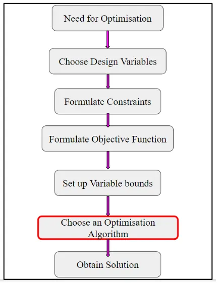
Genetic Algorithm:
- Genetic algorithms (or GAs) are search and optimization techniques used in computing to find true or approximate solutions to specific problems.
- Genetic algorithms are a particular class of evolutionary algorithms that use techniques inspired by evolutionary biology such as inheritance, mutation, selection, and crossover (also called recombination).
- These algorithms are based on Darwin’s principle of “Natural Selection” and “Genetic Inheritance”(Darwin1859)
“Select The Best, Discard The Rest” - GAs search a population of points in parallel, not a single point.
- GAs do not require derivative information or other auxiliary knowledge, only the objective function and corresponding fitness levels influence the directions of search. For this reason, GAs are often called blind search methods.
- GAs use probabilistic transition rules, not deterministic ones. This makes them more robust and applicable to a large range of problems.
- GAs work on an encoding of the parameters set rather than the parameters set itself.
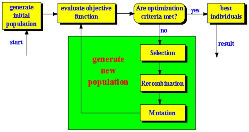
Working Machanism of Genetic Algorithm:
- Population Initialization : Initially many individual solutions are randomly generated to form an initial population.
- Fitness Function( Evaluation): A fitness function quantifies the optimality of a solution so that particular solution may be ranked against all the other solutions.
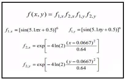
The above function is stalagmite which is used to find out minimum value, but our goal is to find out global maxima for which we are going to multiply the function to find global maxima. the above function has two variable (x,y) so to find the fittest value of function the program do iteration between this two variable.
3. Generation of A New Population :
a.Selection:
During each successive generation, a proportion of the existing population is selected to breed a new generation. Individual solutions are selected through a fitness based process, where fitter solutions (as measured by a fitness function) are typically more likely to be selected. Most functions are designed so that a small proportion of less fit solutions are selected. This helps keep the diversity of the population large, preventing premature convergence on poor solutions.
Example of Roulette Wheel Selection: 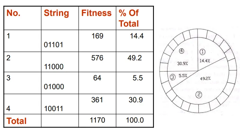
from above pie chart we can see that the string who has highest value of fitness had larger area on pie and all other strngs are distrubuted like that.
b. Reproduction:
The next step is to generate a second generation population of solutions from those selected through genetic operators: crossover (also called recombination), and/or mutation. For each new solution to be produced, a pair of "parent" solutions is selected for breeding from the pool selected previously. By producing a "child" solution using the above operators, a new solution is created which typically shares many of the characteristics of its "parents". The process continues until a new population of solutionsappropriate size is generated. The primary objective of this stage is to determine which solutions are to be preserved and allowed to reproduce and which ones deserve to dieout.
“Selects The Best, Discards The Rest”
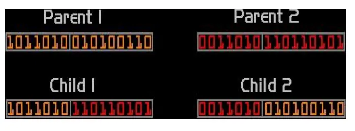
1. Crossover: It is the process in which two chromosomes (strings) combine their genetic material (bits) to produce a new offspring which possesses their both characteristics.The most common type is single point crossover. This process is complex and best understood visually. The children take one section of the chromosome from each parent. The point at which the chromosome is broken depends on the randomly selected crossover point. This particular method is called single point crossover because only one crossover point exists. Crossover does not always occur, however. Sometimes, based on a set probability, no crossover occurs and the parents are copied directly to the new population. The probability of crossover occurring is usually 60% to 70%.
2.Mutation: In order to ensure that the individuals are not all exactly the same, a small chance of mutation is allowed. Change the selected allele either by a small amount or replace it with a new value.(we can remove it)The probability of mutation is usually between 1 and 2 tenths of a percent.
Before : 1 1 0 1 1 0 1 0 0 1 1 0 1 1 1 After : 1 1 0 1 0 0 1 0 0 1 1 0 1 1 1
4.Termination: The process of generation a new population is repeated until a termination condition has been reached.
Common terminating conditions are:
- A solution is found that satisfies maximum criteria.
- Fixed number of generations reached.
- Allocated computation time reached.
- The highest ranking solution's fitness is reaching or has reached a plateau such that successive iterations no longer produce better results.
- Any combinations of the above.
Matlab Program for Genetic Algorithm:
Code for stalagmite Function:
% program for stalegmite function
function [f]= Stalagmite(input_vector);

f1x = (sin(5.1*pi*input_vector(1)+0.5))^6;
f1y = (sin(5.1*pi*input_vector(2)+0.5))^6;

f2x = exp((-4*log(2)*(input_vector(1)-0.0667)^2)/0.64);
f2y = exp((-4*log(2)*(input_vector(2)-0.0667)^2)/0.64);
f  = -(f1x*f1y*f2x*f2y);
end
Code for finding Global Maxima:
% Program for finding the global maxima of stalagmite function by genetic algorithm
clear all
close all
clc
% Input variable
x = linspace(0,0.6,150);
y = linspace(0,0.6,150);
% Number of iteration
num_cases = 50
% combing the input parameters
 [xx,yy] = meshgrid(x,y);
%Calculating Stalagmite function and equating to vector f
  for i = 1:length(xx)
      for j = 1:length(yy)
          input_vector(1)=xx(i,j);
          input_vector(2)=yy(i,j);
      f(i,j) = Stalagmite(input_vector);
      end
  end
tic
%Study 1 - statistical behaviour with unbounded inputs
for k=1:num_cases
    [input1,fopt1(k)] = ga(@Stalagmite,2);
    xopt1(k) = input1(1);
    yopt1(k) = input1(2);
end
time = toc
subplot(2,1,1)
hold on
surfc(x,y,-f)
shading interp
plot3(xopt1,yopt1,-fopt1,'marker','o','markersize',5,'markerfacecolor','r')
title('statistical behaviour with unbounded inputs')
subplot(2,1,2)
plot(-fopt1)
xlabel('iteration')
ylabel('function maximum')

%Study 2 - statistical behaviour with bounded inputs
tic
for l=1:num_cases
    [input2,fopt2(l)] = ga(@Stalagmite,2,[],[],[],[],[0;0],[0.6;0.6]);
    xopt2(l) = input2(1);
    yopt2(l) = input2(2);
end
time2 = toc
figure(2)
subplot(2,1,1)
hold on
surfc(x,y,-f)
shading interp
plot3(xopt2,yopt2,-fopt2,'marker','o','markersize',5,'markerfacecolor','r')
title('statistical behaviour with bounded inputs')
subplot(2,1,2)
plot(-fopt2)
xlabel('iteration')
ylabel('function maximum')


%studt3-statistical behaviour with inceasing ga iteration
options = optimoptions('ga')
options = optimoptions(options,'populationsize',170);

tic
for m=1:num_cases
    [input3,fopt3(m)] = ga(@Stalagmite,2,[],[],[],[],[0;0],[0.6;0.6],[],[],options);
    xopt3(m) = input3(1);
    yopt3(m) = input3(2);
end
time3 = toc
figure(3)
subplot(2,1,1)
hold on
surfc(x,y,-f)
shading interp
plot3(xopt3,yopt3,-fopt3,'marker','o','markersize',5,'markerfacecolor','r')
title('statistical behaviour with inceasing ga iteration')
subplot(2,1,2)
plot(-fopt3)
xlabel('iteration')
ylabel('function maximum')
Explanation of Code:
- First of all using clear all , close all and clc commands for making sure only the program variables are used in the code and all other get erased by using this command.
- The search space of ga is defined using linspace command, from this command we can understand that the x and y array value should be in between 0 – 0.6, here 150 values are used as search space.
- The no. of iterations for ga is defined as num_cases = 50
- By using meshgrid command we can create a 2D plot with the arrary of x and y defined above
- For loop is used to give inputs to stalagmite function inputs which means while running 50 iterations the value changes
- Case 1 – Statistical behaviour with unbounded inputs : In this the optimum values for the inputs taken for each iterations with the help of a for loop
- Study timers commands tic and toc commands are used
- the ga syntax used first study (unbounded inputs)
f=ga(fun,nvars) - Plotting commands
- Figure command is used for opening a figure window and subplot command is used to get multiple plot in one figure window.
- Plot3 command is used for getting the surface as 3D
- Then the title command is used for getting title for the plot also labelled
- In second study, the same parameters are used only the difference is in using the syntax of ga ie, upper and lower bounds are used in second study.
- the ga syntax used in second study (Upper & Lower Bounded Inputs )
f = ga(fun,nvars,A,b,Aeq,beq,lb,ub) - In the case of third study the plotting commands are used as same above but the suntax of ga changed by using optimoptions and increased iterations/population size to 170.
- the ga syntax used third study (Increases iterations/population size using Optimoptions)
f = ga(fun,nvars,A,b,Aeq,beq,lb,ub,nonlcon,IntCon,options)
Input Arguments:
- fun — Objective function(function handle | function name)
- nvars — Number of variables(positive integer)
- A — Linear inequality constraints(real matrix)
- b — Linear inequality constraints(real vector)
- Aeq — Linear equality constraints(real matrix)
- beq — Linear equality constraints(real vector)
- lb — Lower bounds([] (default) | real vector or array)
- ub — Upper bounds([] (default) | real vector or array)
- nonlcon — Nonlinear constraints([] (default) | real vector or array)
- IntCon — Integer variables(vector of positive integers)
- options — Optimization options(output of optimoptions | structure)
Outputs:
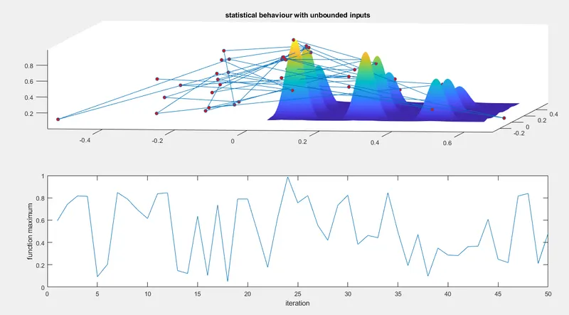
1.statistical behaviour with unbounded inputs
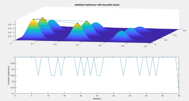
2.statistical behaviour with bounded inputs
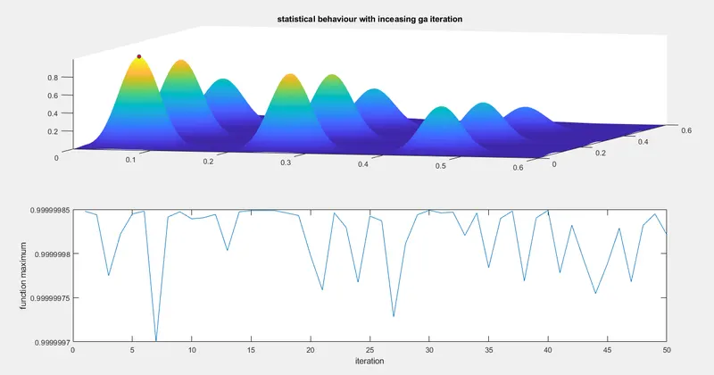
3.statistical behaviour with inceasing ga iteration:
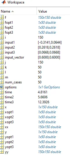
4. Workspace:
Conclusion:
From above graph we can say that know that in case 1 we plot the graph with unbounded conditions with less number of iterations so we get all values. In case 2 we given the bounded conditions with can limit the search space within the defined limit. In case 3 we increased population size with bounded conditions so we get only one global maxima as shown in above graph.But as we go on increasing interations the time for computing is also go on increasing. Genetic algorithms used in a many problem solving and applications in medical, image processing , weather prediction and earth science and so many fields as well the algorithm continue to grow and be more optimal.
Reference: