Solving second order ODEs using MATLAB

Aim: Plotting the graph for the second-order differential equation of a pendulum and also doing animation by using MATLAB program.

Objectives:

1. Understanding of pendulum concept
2. Studying the second ODE of the pendulum
3. Programming in MATLAB for animating the motion of the pendulum

Theory:

A pendulum is a body suspended from a fixed support so that it swings freely back and forth under the influence of gravity. When a pendulum is displaced sideways from its resting, equilibrium position, it is subject to a restoring force due to gravity that will accelerate it back toward the equilibrium position. When released, the restoring force acting on the pendulum's mass causes it to oscillate about the equilibrium position, swinging it back and forth. The mathematics of pendulums is in general quite complicated. Simplifying assumptions can be made, which in the case of a simple pendulum allow the equations of motion to be solved analytically for small-angle oscillations.

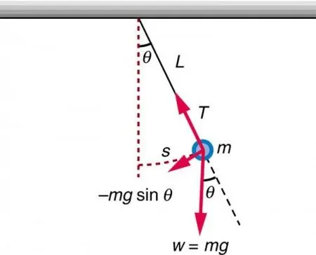
The second order differential equation of pendulum is as follows

`(d^2theta)/dt^2+b/m*(d theta)/(dt)+g/L*sin(theta)=0`

Where as,

b = Dampinmg Coefficient

m = mass of the ball in kg

g = gravity in m/s2

L = Length of pendulum in m

Now for programing this in MATLAB we have to divide this second ODE in first order equations which is as follows,

Let's assume,

`theta=theta1` ..............................................eq(1)

and `(d theta)/dt=(d theta1)/dt=theta2`...........eq(2)

We will get SODE is as follows,

`(d^2theta1)/dt^2+b/m(d theta1)/(dt)+g/L*sin(theta1)=0`

`(d theta2)/dt+b/m*theta2+g/L*sin(theta1)=0` ..............eq(3)

from eq(2) and eq(3) we get

`(d theta1)/dt=theta2`

and `(d theta2)/dt=-b/m*theta2-g/L*sin(theta1)`

from this two equation we can make a matrix to solve the program which is as follows,

`d/dt((theta1)/(theta2))=[(theta2)/(-b/m*theta2-g/L*sin(theta1))]`..........................eq(4)

Code Explanation:

Code 1: Animation of pendulum

% Program for animation of second ODE of pendulum
clear all 
close all
clc

% InputParameters
%Dampinmg Coefficient
b=0.05;
% Length of pendulum in m
g=9.81;
%gravity in m/s2
l=1;
%mass of the ball in kg
m=1;

% input conditions
theta_0 = [0;2];
% time points
t_span = linspace(0,20,500);

% solve ODE
[t,result] = ode45(@(t,theta) ode_func(t,theta,b,g,l,m),t_span, theta_0);
% plotting of results
%Plot for displacement curve 
plot(t,result(:,1),'color','g')
hold on 
% Plot for Angular velocity
plot(t,result(:,2),'color','r')
xlabel('time')
ylabel('plot')
legend('Displacement','Velocity')

% coding for animation of pandulem 
ct = 1; 
for i = 1:length(result(:,1))  
    x0 = 0;  
    y0 = 0;  
    x1 = -l*sin(result(i,1));  
    y1 = -l*cos(result(i,1));  
    figure(2) 
    % PLot for base line
    plot([-0.5 0.5],[0 0],'linewidth',5,'color','b')  
    hold on
    title('Animation of Pendulum')
    %Plot for string of pendulum
    plot([x0 x1],[y0 y1],'linewidth',3,'color','g')
    % Plot for Sphere of pendulum
    plot([x1],[y1],'o','MarkerSize',20,'MarkerFaceColor','r','MarkerEdgeColor','r') 
    axis([-2 2 -2 2])
    grid on
    M(ct) = getframe(gcf);
    hold off
    ct = ct + 1; 
   
    
end
 % saving the animation video file
 movie(M)
 videofile = VideoWriter('second_order_ode.avi','uncompressed AVI')
 open(videofile)
 writeVideo(videofile,M)
 close(videofile)

Explanation:

1. In the first step, we define the basic parameters of the pendulum such as length, mass, damping coefficient, etc.
2. In a second step, we have to define the initial condition of a pendulum which is displacement and angular velocity.
3. Now we have to define the function for the second ODE for pendulum which is shown in eq(4) above, so the function is as shown in code 2

code 2: Defining the function of the second ODE of the pendulum

% Program for defining the function 
function [dtheta_dt] = ode_func(t,theta,b,g,l,m);

theta1 = theta(1);
theta2 = theta(2);
dtheta1_dt = theta2;
dtheta2_dt = -(b/m)*theta2-(g/l)*sin(theta1);
dtheta_dt = [dtheta1_dt ; dtheta2_dt];
end​

1. Next step we have to plot the displacement and angular velocity curve by using plot and hold on command to get the combined result of both w.r.t. time
2. Now for doing an animation of the second ODE of the pendulum we have to define loop counter variable and for loop to each motion of the pendulum.
3. Last step is to save the movie or animation in .avi format by using commands.

Output:

1. Displacement and angular velocity graph w.r.t. time
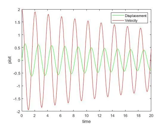
2. Animation of Second ODE Pendulum Video Link https://youtu.be/LkU8aigJ8KU

Conclusion:

So from this project, we can conclude that by varying position(theta) of any pendulum with fixed parameters we can plot the relationship of displacement and angular velocity with respect to time which is shown in the above graph, and also by dividing the second ODE into the first ODE we can do MATLAB program and get the trajectory path of the pendulum and this can be used for any application to see the trajectory path of an object.

Reference:

https://en.wikipedia.org/wiki/Pendulum_(mathematics)