Curve Fitting by split wise method

Aim: To plot curve fit for linear and cubic order and compare this curve with original data curve to get curve fit parameters and also do curve fitting by split wise method and compare all results to get best curve fit by using MATLAB Program.

Objectives :

1. Studying about curve fitting and it's methods and parameters.
2. Compare orignal and curve fit curves for linear polynomial and calculate curve fit parameters.
3. Compare orignal and curve fit curves for cubic polynomial and calculate curve fit parameters.
4. Compare orignal and curve fit curves for spilt wise method and calculate curve fit parameters.
5. compare curve fit parameters of linear polynomial, cubic polynomial and split wise method to get best method for curve fitting.

Theory:

Curve fitting is an optimization problem that finds a line that best fits a collection of observations. It is easiest to think about curve fitting in two dimensions, such as a graph.

Consider that we have collected examples of data from the problem domain with inputs and outputs.

The x-axis is the independent variable or the input to the function. The y-axis is the dependent variable or the output of the function. We don’t know the form of the function that maps examples of inputs to outputs, but we suspect that we can approximate the function with a standard function form.Curve fitting involves first defining the functional form of the mapping function (also called the basis function or objective function), then searching for the parameters to the function that result in the minimum error. Once fit, we can use the mapping function to interpolate or extrapolate new points in the domain. It is common to run a sequence of input values through the mapping function to calculate a sequence of outputs, then create a line plot of the result to show how output varies with input and how well the line fits the observed points.

The key to curve fitting is the form of the mapping function.

A straight line between inputs and outputs can be defined as follows:

• y = a * x + b

Where y is the calculated output, x is the input, and a and b are parameters of the mapping function found using an optimization algorithm.

This is called a linear equation because it is a weighted sum of the inputs.

In a linear regression model, these parameters are referred to as coefficients; in a neural network, they are referred to as weights.

This equation can be generalized to any number of inputs, meaning that the notion of curve fitting is not limited to two-dimensions (one input and one output), but could have many input variables.

For example, a line mapping function for two input variables may look as follows:

• y = a1 * x1 + a2 * x2 + b

The equation does not have to be a straight line.

We can add curves in the mapping function by adding exponents. For example, we can add a squared version of the input weighted by another parameter:

• y = a * x + b * x^2 + c

This is called polynomial regression, and the squared term means it is a second-degree polynomial.

So far, linear equations of this type can be fit by minimizing least squares and can be calculated analytically. This means we can find the optimal values of the parameters using a little linear algebra.

We might also want to add other mathematical functions to the equation, such as sine, cosine, and more. Each term is weighted with a parameter and added to the whole to give the output; for example:

• y = a * sin(b * x) + c

Adding arbitrary mathematical functions to our mapping function generally means we cannot calculate the parameters analytically, and instead, we will need to use an iterative optimization algorithm.

This is called nonlinear least squares, as the objective function is no longer convex (it’s nonlinear) and not as easy to solve.

-Their are different methods to get good fit curve but we are using least square method because we are having ploynomial equations.

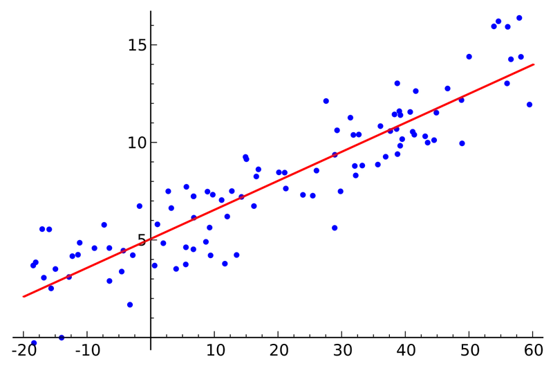
figure1

-Parameters of least square method for finding good fit curve are as follows:

1. The Sum of Square of Error(SSE)

2. R-Square

3. Adjusted R-Square

4. Root Mean Squared Error(RMSE)

Let' Discuss this term more briefly as follows for identifying

Lets consider the linear equation y=f(x) and set point for best fit are (x1,y1),(x2,y2),(x3,y3)...........(xn.yn) so for this equation the curve of best fit is as shown in figure1

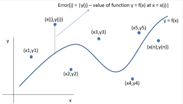
figure2

Suppose each of these n points has an individual error (difference in y co-ordinate values).

The error for a general "i" point can be given by the function,

Error = |y(i)- value of f(x) at x(i)|

Error = `|y(i)-f(x(i))|`

squaring this error to remove the module sign and add all the 'n' terms to get summation of all the term as follows

SSE(Sum of Square Error) = `overset(n)underset(i=1)sum`Error`(i)^2`

2. R-Square:

This quantity measures how successful the fit is in explaining the variation of the data.Put another way, R-square is the square of the correlation between the response values and the predicted response values. It is also called the square of the multiple correlation coefficient and the coefficient of multiple determination.

The range of R-Square is between 0 to 1.

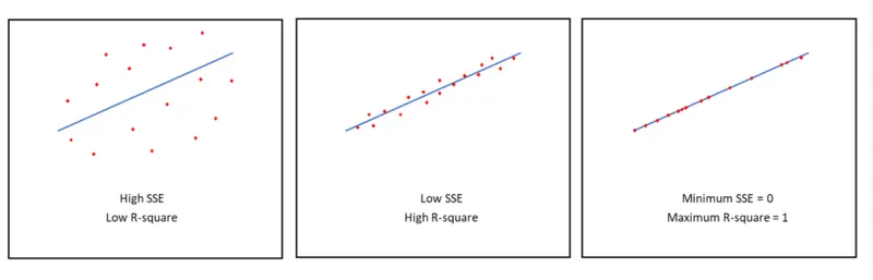
figure3

As shown in figure3 we can say that SSE is inversly propertional to R_Square.

The formula for calculation of R-Square is as follows

`R^2=(SSR)/(SST)`

Where as ,

SSR = Sum of Regression

SSR for y=f(x) curve can be calculated as follows,

SSR = `overset(n)underset(i-1)sum(f(x(i))-Mean)^2`

and we know SSE is as follows,

SSE = `overset(n)underset(i=n)sum(y(i)-f(x(i)))^2`

Therefor SST(Sum of Square Term) is as follows,

SST = SSR+SSE

3.Adjusted R-Square:

First up all why we using this Adjusted R-Square instead of R- Square is because of following reasons,

• Every time you add a predictor to a model, the R-squared increases, even if due to chance alone. It never decreases. Consequently, a model with more terms may appear to have a better fit simply because it has more terms.
• If a model has too many predictors and higher order polynomials, it begins to model the random noise in the data. This condition is known as overfitting the model and it produces misleadingly high R-squared values and a lessened ability to make predictions.

Now Let's study about overfitting of the curve,

Overfitting Curve:Overfitting is a term used in statistics that refers to a modeling error that occurs when a function corresponds too closely to a particular set of data. As a result, overfitting may fail to fit additional data, and this may affect the accuracy of predicting future observations.

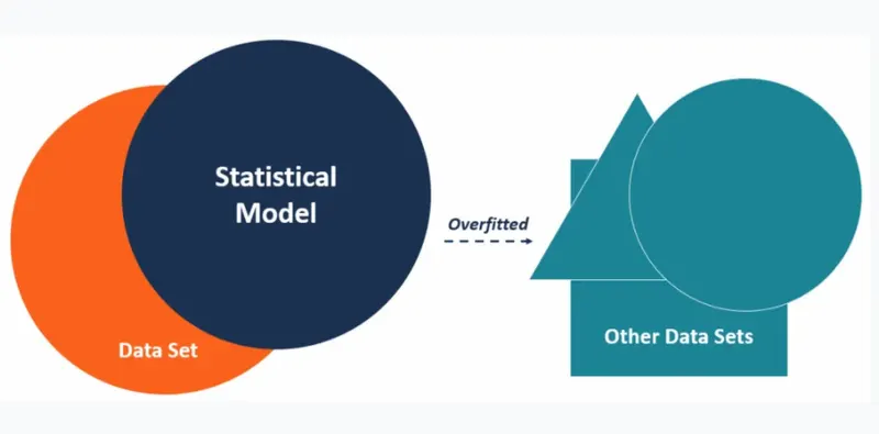
figure4

Overfitting can be identified by checking validation metrics such as accuracy and loss. The validation metrics usually increase until a point where they stagnate or start declining when the model is affected by overfitting. During an upward trend, the model seeks a good fit, which, when achieved, causes the trend to start declining or stagnate.

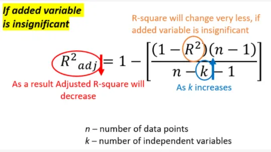
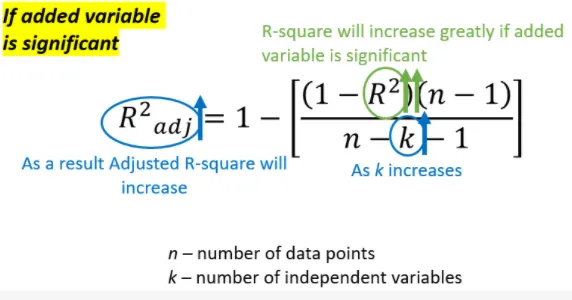
The formula for calculation of adjusted R-Square is as follows,

`( R^2)_(Adj) = 1-[((1-R^2)*(n-1))/(n-k-1)]`

Where as,

k = Number of independent variable

n = Number of datapoints

Here their are two possibilities either the added variable is significant or the variable is insignificant according to that the value R-Square changes as follows,

for insignificant variable:

for significant variable:

4. RMSE(Root Mean Square Error)

Root Mean Square Error (RMSE) is the standard deviation of the residuals (prediction errors). Residuals are a measure of how far from the regression line data points are; RMSE is a measure of how spread out these residuals are. In other words, it tells you how concentrated the data is around the line of best fit. Root mean square error is commonly used in climatology, forecasting, and regression analysis to verify experimental results.

`RSME = sqrt((underset(i=1)overset(n)(sum)(y(i)-f(x(i)))^2)/n) = sqrt((SSE)/n)`

Using these four quantities Matlab effectively deduces the goodness of fit, typically is R-square is greater than 0.95 the fit is assumed to be good.

MATLAB Prgram for Linear Order Equation:

%Program for Linear order equation for curve fitting  
clear all 
close all
clc
%Data set for plotting curve 
cp_data = load('data');
% Independent variable 
temperature = cp_data(:,1);
% Dependent variable
cp = cp_data(:,2);

%curve fit for Linear equation
% cp = a*T+b
%Finding unknown coefficent a,b by using polyfit command

co_eff = polyfit(temperature,cp,1);
% calculation of pradicted_cp by using polyval command
pradicted_cp =  polyval(co_eff,temperature);

% calculations of good fit curve parameters
for i= 1:length(cp);
    x(i) = (pradicted_cp(i)-cp(i))^2;
    y(i) = (pradicted_cp(i)-mean(cp))^2;
end
% Calculation of Sum of Square Error(SSE)
SSE = sum(x)
% Calculation of sum of square Regression(SSR)
SSR = sum(y)
% Calculation of R_Square from SSE and SSR
R_square = (SSR/(SSR+SSE))
% Calculation of Adjusted R_Square 
% k = No. of independent variable
k=0;
% n = No. of datapoints
n = length(cp);
Adj_R_Square = 1-(((1-R_square)*(n-1))/(n-k-1))
%Calculation of Root Mean Square Error(RMSE)
RSME = sqrt(SSE/n)
% Displaying whether the curve is good fit or not
if (R_square>0.95);
    disp('Curve is Good Fit')
else 
    disp('Curve is not Good Fit')
end
%compare curve fit data with orignal data
% Plotting of orignal data curve 
plot(temperature,cp,'linewidth',3)
hold on
% Plotting of curve fit data curve
plot(temperature, pradicted_cp, 'linewidth',3,'color','R')
xlabel('Temperature[K]')
ylabel('Spacific Heat[kJ/kgK]')
legend('Orignal Curve','Curve fit')
title('Curve fit for first order equation')
grid on

MATLAB Prgram for cubic Equation:

%Program for Cubic order equation for curve fitting  
clear all 
close all
clc
%Data set for plotting curve 
cp_data = load('data');
% Independent variable 
temperature = cp_data(:,1);
% Dependent variable
cp = cp_data(:,2);

%curve fit for Linear equation
% cp = a*T^3+b*T^2+c*T+d
%Finding unknown coefficent a,b by using polyfit command
co_eff = polyfit(temperature,cp,3);
% calculation of pradicted_cp by using polyval command
pradicted_cp =  polyval(co_eff,temperature);

% calculations of good fit curve parameters
for i= 1:length(cp);
    x(i) = (pradicted_cp(i)-cp(i))^2;
    y(i) = (pradicted_cp(i)-mean(cp))^2;
end
% Calculation of Sum of Square Error(SSE)
SSE = sum(x)
% Calculation of sum of square Regression(SSR)
SSR = sum(y)
% Calculation of R_Square from SSE and SSR
R_square = (SSR/(SSR+SSE))
% Calculation of Adjusted R_Square 
% k = No. of independent variable
k=0;
% n = No. of datapoints
n = length(cp);
Adj_R_Square = 1-(((1-R_square)*(n-1))/(n-k-1))
%Calculation of Root Mean Square Error(RMSE)
RSME = sqrt(SSE/n)
% Displaying whether the curve is good fit or not
if (R_square>0.95);
    disp('Curve is Good Fit')
else 
    disp('Curve is not Good Fit')
end
%compare curve fit data with orignal data
% Plotting of orignal data curve 
plot(temperature,cp,'linewidth',3)
hold on
% Plotting of curve fit data curve
plot(temperature, pradicted_cp, 'linewidth',3,'color','R')
xlabel('Temperature[K]')
ylabel('Spacific Heat[kJ/kgK]')
legend('Orignal Curve','Cubic Curve fit')
title('Curve fit for Cubic order equation')
grid on

Explanation of MATLAB Program:

1. First up all we should have data sets to plot the curve so we have to define the data file location by load command. Remember that file should be saved where the data file is saved.

2. After defining the data on which we are going to plot the curve now we have to define parameters in this case we have defined 'temperature' and 'Spacific Heat' from data file as shown in above program.

3. In ideal condition the spacific heat should be constant during temperature change but real condition it changes due to variables of equation so to calculate change in cp we will do following steps as follows.

4. Now we use 'polyfit' command to calculate the coefficients of the equation, we can define the plotfit command as follows

• p = polyfit(x,y,n) returns the coefficients for a polynomial p(x) of degree n that is a best fit (in a least-squares sense) for the data in y. The coefficients in p are in descending powers, and the length of p is n+1
• [p,S] = polyfit(x,y,n) also returns a structure S that can be used as an input to polyval to obtain error stimates
• [p,S,mu] = polyfit(x,y,n) also returns mu, which is a two-element vector with centering and scaling values. mu(1) is mean(x), and mu(2) is std(x). Using these values, polyfit centers x at zero and scales it to have unit standard deviation, this is required when we are using higher order equation and due to this our curve is disordering then we use this.

5. Now to calculate prdicted spacific heat we use Polyval to evaluate a polynomial for a given set of x values. So, Polyval generates a curve to fit the data based on the coefficients found using polyfit it works as follows,

• y = polyval(p,x) evaluates the polynomial p at each point in x. The argument p is a vector of length n+1 whose elements are the coefficients (in descending powers) of an nth-degree polynomial

6.Now we use for loop to calculate the sum of square error(SSE) and sum of square regression (SSR) by calculating Error as shown in coding

7. After this we calculate good fit parameters which are as follows ,

• R_Square
• Adjusted R_ Square
• Root Mean Square Error(RMSE)

8. Now we conditional statement if else to display whether the is good fit or not we say the if R_Square is greater than 0.95 then display the curve is good fit otherwise curve is not good fit.

9. Now we plot the graph of orignal cp data and pradicted cp dta with repect to temperature by using plot command.

Split Wise Method for curve fitting:

First up all why we are using this split wise method for cuve fitting if we can use different order ploynomial equation for good fit?

anwer to the above question is as follows:

Case1:Overfit - over-doing the requirement for the fit to ‘match’ the data trend (order too high)

Polynomials become more ‘squiggly’ as their order increases. A ‘squiggly’ appearance comes from inflections in function as you can see in below figure5

Consideration #1:
3rd order - 1 inflection point
4th order - 2 inflection points
nth order - n-2 inflection points
Consideration #2:
2 data points - linear touches each point
3 data points - second order touches each point
n data points - n-1 order polynomial will touch each point

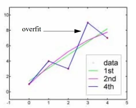
figure5

SO: Picking an order too high will overfit data

General rule: pick a polynomial form at least several orders lower than the number of data points. Start with linear and add order until trends are matched.

Case2:Underfit - If the order is too low to capture obvious trends in the data.

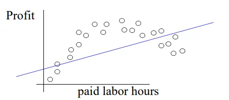
figure6

Straight line will not predict diminishing returns that data shown in figure6.

General rule: View data first, then select an order that reflects inflections, etc

So due to this we have to use split wise method so let's see what will be the results,

MATLAB Program for Split Wise curve fitting method:

% Program for Split wise method for curve fitting 
clear all
close all
clc
% Initial Data sets by split wise methods
cp_data = load('data');
temperature = cp_data(:,1); 
cp = cp_data(:,2);

%calcution by split wise method 
% first set of data points (1,400)
temperature_1= cp_data(1:400,1);
cp_1 = cp_data(1:400,2);
% curve fir for Linear equation
[co_eff_1] = polyfit(temperature_1,cp_1,1)
pradicted_cp_1 = polyval(co_eff_1,temperature_1);

% Second set of data points (401,800)
temperature_2= cp_data(401:800,1);
cp_2 = cp_data(401:800,2);
% curve fir for Linear equation
[co_eff_2] = polyfit(temperature_2,cp_2,1)
pradicted_cp_2 = polyval(co_eff_2,temperature_2);


% Third set of data points (801,1200)
temperature_3= cp_data(801:1200,1);
cp_3 = cp_data(801:1200,2);
% curve fir for Linear equation
[co_eff_3] = polyfit(temperature_3,cp_3,1)
pradicted_cp_3 = polyval(co_eff_3,temperature_3);


% Four set of data points (1201,1600)
temperature_4= cp_data(1201:1600,1);
cp_4 = cp_data(1201:1600,2);
% curve fir for Linear equation
[co_eff_4] = polyfit(temperature_4,cp_4,1)
pradicted_cp_4 = polyval(co_eff_4,temperature_4);

% Fifth set of data points (1601,2000)
temperature_5= cp_data(1601:2000,1);
cp_5 = cp_data(1601:2000,2);
% curve fir for Linear equation
[co_eff_5] = polyfit(temperature_5,cp_5,1)
pradicted_cp_5 = polyval(co_eff_5,temperature_5);

% Sixth set of data points (2001,2400)
temperature_6= cp_data(2001:2400,1);
cp_6 = cp_data(2001:2400,2);
% curve fir for Linear equation
[co_eff_6] = polyfit(temperature_6,cp_6,1)
pradicted_cp_6 = polyval(co_eff_6,temperature_6);

% Seventh set of data points (2401,2800)
temperature_7= cp_data(2401:2800,1);
cp_7 = cp_data(2401:2800,2);
% curve fir for Linear equation
[co_eff_7] = polyfit(temperature_7,cp_7,1)
pradicted_cp_7 = polyval(co_eff_7,temperature_7);

% Eighth set of data points (2801,3200)
temperature_8= cp_data(2801:3200,1);
cp_8 = cp_data(2801:3200,2);
% curve fir for Linear equation
[co_eff_8] = polyfit(temperature_8,cp_8,1)
pradicted_cp_8 = polyval(co_eff_8,temperature_8);
% collecting all data point under one matrix
pradicted_cp = [pradicted_cp_1;pradicted_cp_2;pradicted_cp_3;pradicted_cp_4;pradicted_cp_5;pradicted_cp_6;pradicted_cp_7;pradicted_cp_8];
Temperature = [temperature_1;temperature_2;temperature_3;temperature_4;temperature_5;temperature_6;temperature_7;temperature_8];
% calculations of good fit curve parameters
for i= 1:length(cp);
    x(i) = (pradicted_cp(i)-cp(i))^2;
    y(i) = (pradicted_cp(i)-mean(cp))^2;
end
% Calculation of Sum of Square Error(SSE)
SSE = sum(x)
% Calculation of sum of square Regression(SSR)
SSR = sum(y)
% Calculation of R_Square from SSE and SSR
R_square = (SSR/(SSR+SSE))
% Calculation of Adjusted R_Square 
% k = No. of independent variable
k=0;
% n = No. of datapoints
n = length(cp);
Adj_R_Square = 1-(((1-R_square)*(n-1))/(n-k-1))
%Calculation of Root Mean Square Error(RMSE)
RSME = sqrt(SSE/n)
% plotting of orignal curve fir
plot(temperature,cp,'linewidth',5,'color','r')
hold on
plot(Temperature,pradicted_cp,'linewidth',3,'color','g')
grid on
xlabel('Temperature')
ylabel('Spacific Heat')
legend('orignal curve','Split wise method curve')
title('split wise method for curve fitting')
% Displaying whether the curve is good fit or not
if (R_square>0.95);
    disp('Curve is Good Fit')
else 
    disp('Curve is not Good Fit')
end

Explanation of program:

1. The program is same as linear order equation we are just splitting the data in different sets so that for each set we can get curve

2. we have splitted the data into 8 set as you can see in progam.

3. In this method as we have splitted the data in 8 sets so we get 8 different temperature and pradicted spacific heat.

4. Now we collect all temperature and pradicted spacific heat under one matrix as shown in program due to this we can plot the curve easily.

5. After this we calcalute parameters of good fit curve and define conditional statement for displaying whether the curve is good fit or not.

6.Now we plot the grapth between cp and pradicted cp with respect to temperature and compare the graph of orignal data set and splittted data set curve.

Output:

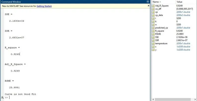
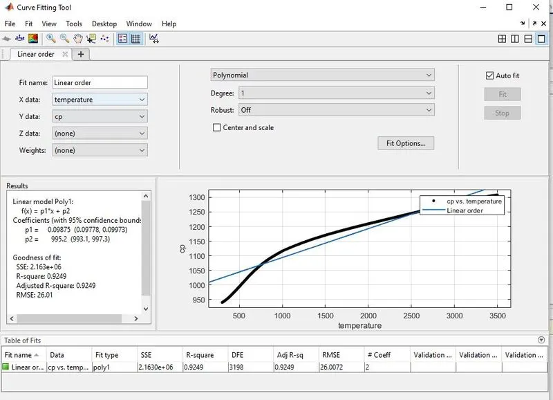
1. For Linear Order Equation:

a. Linear Order curve fit parameters by program :

b.Linear Order Curve fit parameters by curve fit tool:

c. Grapth between orignal curve and linear order curve fit:

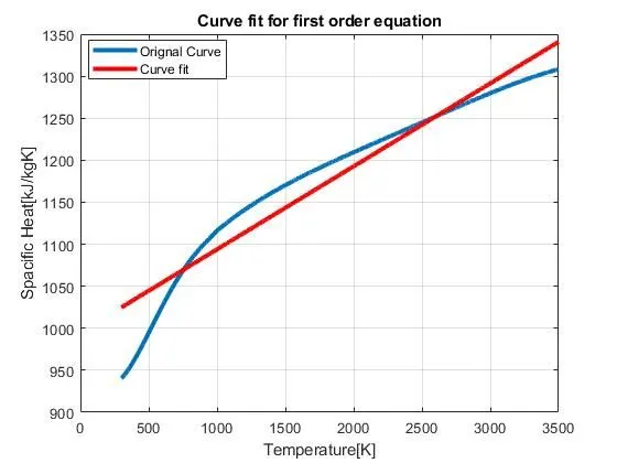
figure7

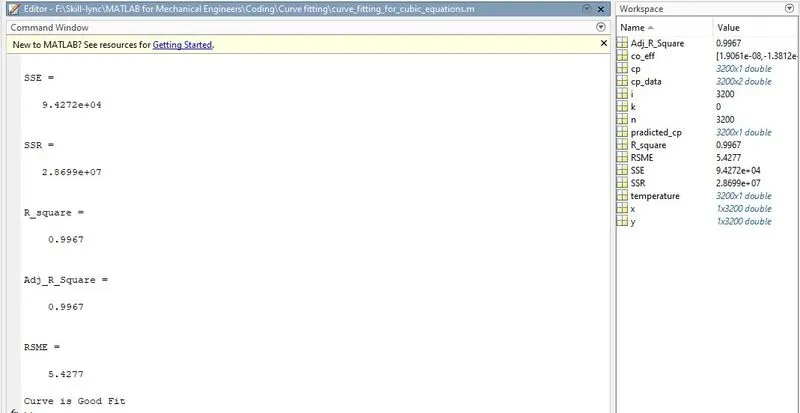
2.For cubic order Equation:

a.Cubic Order curve fit parameters by program:

b.Cubic Order Curve fit parameters by curve fit tool:

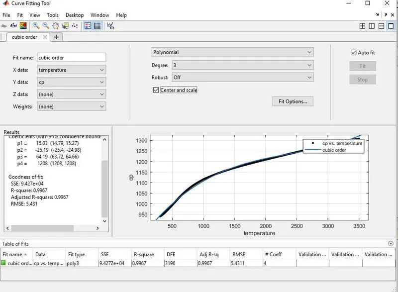
c. Grapth between orignal curve and Cubic order curve fit:

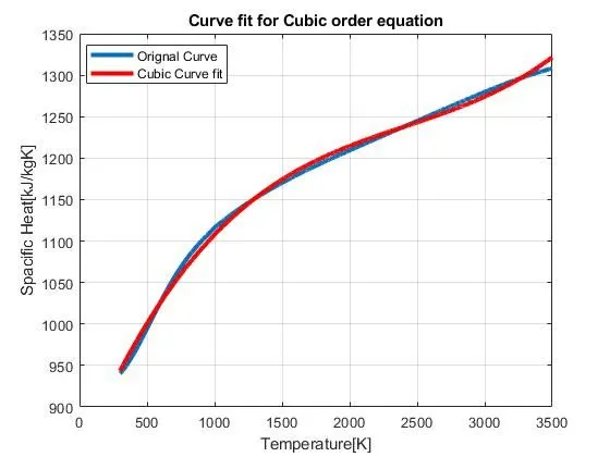
figure8

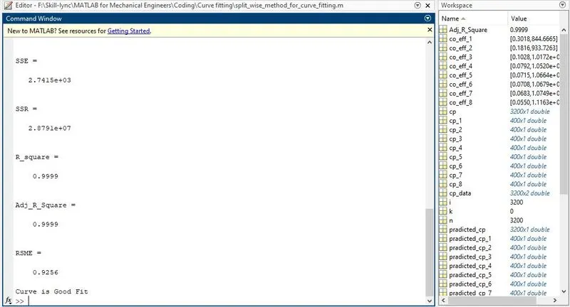
3.Split wise method for curve fitting:

a.Cubic Order curve fit parameters by program:

b. Grapth between orignal curve and Cubic order curve fit:

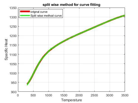
figure9

conclusion:

From above outputs and graphs we can conclude that if we incerese order of equation we can get a good curve fit but if we go on increasing the value of order of equation then at one point we will get disorder equation means points are overlapping which is called overfit already explanied in above section, so avoid this overfit we can use split wise method in which we just split the curve and do calculation of parameters for particular set and later on combine them to get full curve which is good fit curve as shown in figure9.

Reference:

• https://en.wikipedia.org/wiki/Curve_fitting
• https://skill-lync.com/projects/Curve-Fitting-and-criterion-to-choose-best-fit-41860
• https://in.mathworks.com/help/matlab/ref/polyfit.html
• https://in.mathworks.com/help/matlab/ref/polyval.html
• https://www.iiserpune.ac.in/~bhasbapat/phy221_files/curvefitting.pdf

Q&A:

1.How to make a curve fit perfectly?

In order to make perfect fit, we must consider error estimates.

2.How to get the best fit?

Perfect fit means, the curve should fit the original curve without showing any errors (such as centering and scaling erros) in that perticular degree of polynomial. Perfect fit can always be a best fit but best fit can not be a perfect fit.

3.What could be done to improve the cubic fit?

To improve the cubic fit we should Call polyfit with 3 outputs such as [p,S,mu] = polyfit(x,y,n) also returns mu, which is a two-element vector with centering and scaling values. mu(1) is mean(x), and mu(2) is std(x). Using these values, polyfit centers x at zero and scales it to have unit standard deviation, this is required when we are using higher order equation and due to this our curve is disordering, then we use this.