Rankine cycle Simulator using MATLAB
Aim: To do programming for the Rankin cycle simulator by using the MATLAB program and plot the graph for T-S and H-S.
Objective:
- To study about Rankine cycle.
- Study about different regions present in T-s graph.
- Study about different states present in the Rankine cycle
- Learn how to do programming for the Rankine cycle simulator.
Theory:
Rankine Cycle: The Rankine cycle is an idealized thermodynamic cycle describing the process by which certain heat engines, such as steam turbines or reciprocating steam engines, allow mechanical work to be extracted from a fluid as it moves between a heat source and heat sink.
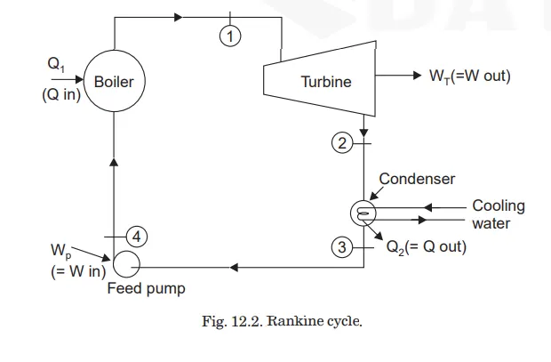
The above Rankine cycle figure contains four different processes which are as follows:
- 1-2 = In process 1-2 dry saturated vapor expands through a turbine generating power. This decreases the temperature and pressure of the vapor and some condensation may occur.[Isentropic Expansion]
- 2-3 = In process 2-3 wet vapor enters a condenser, where it is condensed at constant pressure to become saturated liquid.[Heat rejection at constant pressure]
- 3-4 = In process 3-4 fluid is pumped from low to high pressure.[Isentropic compression]
- 4-1 = In process 4-1 high-pressure liquid enters the boiler, where it is heated at constant pressure by an external heat source to become a dry saturated vapor.[Heat addition at constant pressure]
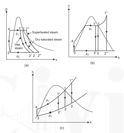
Applying steady flow energy equation (S.F.E.E.) to boiler, turbine, condenser, and pump :
(i) For boiler (as control volume), we get
hf4 + Q1 = h1
Q1 = h1 – hf4
(ii) For turbine (as control volume), we get
h1 = WT + h2, where WT = turbine work
WT = h1 – h2
(iii) For condenser, we get
h2 = Q2 + hf3
Q2 = h2 – hf3
(iv) For the feed pump, we get
hf3 + WP = hf4 , where, WP = Pump work
WP = hf4 – hf3
(v) efficiency of Rankine cycle is given by
`eta_(Ranki n e) = (W_(n et))/Q_(i n) = (W_T-W_P)/Q_(i n)`
(vi) Back work ratio
`W_(BWR) = W_T/W_P`
(vii) for isentropic expansion
`T_2/T_1 = (P_2/P_1)^(1-(1/gamma))`
(ix) if the state point 2 is in the superheated region
to calculate enthalpy:
`H = H_g +c_p(T-T_(sat))`
to calculate temperature:
`T2=(T_(sat)+273.15)*e^(((S2-Sg_2)/(C_p)))`
Program for Rankine cycle simulator:
% progrsm for rankine cycle simulator
clear all
close all
clc
%Tsat_p	Saturation temperature
%hV_p	Saturated vapour enthalpy
%hL_p	Saturated liquid enthalpy
%hV_T	Saturated vapour enthalpy
%hL_T	Saturated liquid enthalpy
%h_pT	Entalpy as a function of pressure and temperature.
%h_ps	Entalpy as a function of pressure and entropy.
%vV_p	Saturated vapour volume
%vL_p	Saturated liquid volume
%vV_T	Saturated vapour volume
%vL_T	Saturated liquid volume
%v_pT	Specific volume as a function of pressure and temperature.
%v_ph	Specific volume as a function of pressure and enthalpy
%v_ps	Specific volume as a function of pressure and entropy.
%sV_p	Saturated vapour entropy
%sL_p	Saturated liquid entropy
%sV_T	Saturated vapour entropy
%sL_T	Saturated liquid entropy

%inputs parameters
P1 = input('Enter the Pressure at the Turbine Inlet (bar)= ');
T1 = input('Enter the Temperature at the Turbine inlet (°C)= ');
P2 = input('Enter the Pressure at the Condenser (bar)= ');
%getting Cp and cv values from XSteam
%Cp and Cv assumed to  not change with temperature to make problem simple
% for vapur
high_cpV= XSteam('CpV_p', P1);
low_cpV=XSteam('CpV_p', P2);
% for liquid
high_cpL= XSteam('CpL_p', P1);
low_cpL=XSteam('CpL_p', P2);
%Getting important parameters from XSteam
%for high pressure
Tsat_p1 = XSteam('Tsat_p', P1);
Sg_1 = XSteam('sV_p', P1);
Sf_1 = XSteam('SL_p', P1);
Sgf_1 = Sg_1 - Sf_1;
Hf_1 = XSteam('hL_p', P1);
Hg_1 = XSteam('hV_p', P1);
Hfg_1 = Hg_1 - Hf_1;
%for low pressure
Sg_2 = XSteam('sV_p', P2);
Sf_2 = XSteam('SL_p', P2);
Sfg_2 = Sg_2 - Sf_2;
Tsat_p2 = XSteam('Tsat_p', P2);
Hf_2 = XSteam('hL_p', P2);
Hg_2 = XSteam('hV_p', P2);
Hfg_2 = Hg_2 - Hf_2;

%% State point 1
H1 = XSteam('h_pt', P1, T1);   % enthalpy of the point
S1 = XSteam('s_pt', P1, T1);   % entropy of the point
%% State point 2
S2 = S1;
%predicting location of point 2 in T-s
if(Sf_2>=S2<=Sg_2)
    X2 = (S2 - Sf_2) / (Sfg_2);   % Dryness Fraction at state point 2
else
    X2=1;                          % for vapour State
end
T2=Tsat_p2;
H2 = Hf_2 + X2 * Hfg_2;

%% State point 3
% Assuming no subcooling in condensor
P3 = P2;
V3 = XSteam('vL_p', P3);
T3 = Tsat_p2;    %no subcooling assumed
H3 = Hf_2;        % enthalpy at state point 3
S3 = Sf_2;        % entropy at state point 3

%% State point 4
P4 = P1;    % pressure at point 4
S4 = S3;    % entropy at state point 4
Wp = V3 * (P4 - P3) * 100; % work done by pump
H4 = Wp + H3;              % Enthalpy at state point 4
% to cal T4 s4=s3=sf1-high_cpL*ln(t1s/t4)
A=exp((Sf_1-S4)/high_cpL);  %Use exp instead of Exp to take input as double
T4= (Tsat_p1)/A;

%% Work done, heat, SSC and efficiency calculations
Wt = H1 - H2; % work done by turbine
Wnet = Wt - Wp;  % net work done by systeam
Qin = H1 - H4;   % heat addition
eff_thermal = (Wnet / Qin)*100 ;    % Effieciency
% to calculate back work ratio
Wbr = Wp/Wt;
SSC = 3600 / Wt;    % Specific steam consuption
%% Calculation for plotting Liquid and Vapour line
temp = linspace(1,374.14, 1000);
for i = 1 : length(temp)
     H_L(i) = XSteam('hL_T', temp(i));
     H_V(i) = XSteam('hV_T', temp(i));
     S_L(i) = XSteam('sL_T', temp(i));
     S_V(i) = XSteam('sV_T', temp(i));
end
%% for printing all values
fprintf('                        SIMULATOR OF RANKINE CYCLE  nn')
fprintf('1-2  Isentropic Expansion in the Turbine n')
fprintf('2-3  Constant Pressure Heat Rejection by the Condenser n')
fprintf('3-2  Isentropic Compression in the Pumpn')
fprintf('4-1  Constant Pressure Heat Addition by the Boilern')

disp('                               RESULTS                   ')
fprintf('At state point 1                                     '); fprintf('At state point 4 n')
fprintf('P1 = %f Bar                                   ', P1); fprintf('P4 = %f Bar n', P4);
fprintf('T1 = %f °C                                   ', T1); fprintf('T4 = %f °C n', T4)
fprintf('H1 = %f kJ/kg                               ', H1); fprintf('H4 = %f kJ/kg n', H4)
fprintf('S1 = %f kJ/kgK                                 ', S1); fprintf('S4 = %f kJ/kgK nn', S4)

fprintf('At state point 2                                     '); fprintf('S.S.C is : %f kg/kWh n ', SSC)
fprintf('P2 = %f Bar v                                 ', P2);   fprintf('Work by turbine = %f kJ/kg n', Wt)
fprintf('T2 = %f °C                                    ', T2);    fprintf('Work by compressor = %f kJ/kg n', Wp)
fprintf('H2 = %f kJ/kg                               ', H2);     fprintf('Net Wok done = %f kJ/kg n', Wnet)
fprintf('S2 = %f kJ/kgK                                 ', S2);  fprintf('Back work ratio = %f n',Wbr)
fprintf('X2 = %f                                        ', X2);  fprintf('Thermal efficiency = %f percent n', eff_thermal);

disp('At state point 3')
fprintf('P3 = %f Bar n', P3)
fprintf('T3 = %f °C n', T3)
fprintf('H3 = %f kJ/kg n', H3)
fprintf('S3 = %f kJ/kgK nn', S3)
%% Ploting T - S and H - S graph

figure(1) % plot for T-S graph
hold on
plot([S1 S2], [T1 T2], 'g', 'linewidth', 1)
text(S1,T1,' 1')
text(S2,T2,' 2')
if (X2>1)
plot([S2 Sg_2], [T2 Tsat_p2], 'g', 'linewidth', 1)
text(Sg_2,Tsat_p2,' 2s')
end
if (X2>1)
plot([Sg_2 S3], [Tsat_p2 T3], 'g', 'linewidth', 1)
text(S3,T3,' 3')
else
plot([S2 S3],[T2 Tsat_p2],'g','linewidth',1)
text(S3,T3,'3')
end
plot([S3 S4], [T3 T4], 'g', 'linewidth', 1)
text(S4,T4,' 4')
plot([S4 Sf_1], [T4 Tsat_p1], 'g', 'linewidth', 1)
text(Sf_1,Tsat_p1,' 4s')
plot([Sf_1 Sg_1], [Tsat_p1 Tsat_p1], 'g', 'linewidth', 1)
text(Sg_1,Tsat_p1,' 1s')
plot([Sg_1 S1], [Tsat_p1 T1], 'g', 'linewidth', 1)
plot(S_L, temp, 'b', 'linestyle','-','linewidth', 2)
plot(S_V, temp, 'b', 'linestyle','-','linewidth', 2)
%marking direction
title('T-S Diagram of Ideal Rankine Cycle','FontSize', 20)
ylabel('Temprature (°C)')
xlabel('Specific Entropy (kJ/kgK)')

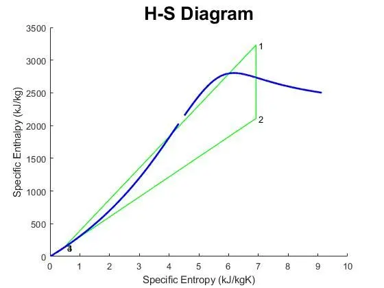
figure(2) % plot for H-S graph
hold on
plot([S1 S2], [H1 H2], 'g', 'linewidth', 1);
text(S1,H1,' 1')
plot([S2 S3], [H2 H3], 'g', 'linewidth', 1);
text(S2,H2,' 2')
plot([S3 S4], [H3 H4], 'g', 'linewidth', 1);
text(S3,H3,' 3')
plot([S4 S1], [H4 H1], 'g', 'linewidth', 1);
text(S4,H4,' 4')
plot(S_L, H_L, 'b','linestyle','-', 'linewidth', 2)
plot(S_V, H_V, 'b','linestyle','-', 'linewidth', 2)
title('H-S Diagram', 'FontSize', 20)
ylabel('Specific Enthalpy (kJ/kg)')
xlabel('Specific Entropy (kJ/kgK)')
Explanation of Code:
1. first of all we define the process and input parameters with the fprintf and input command, in input parameters we have an inlet pressure of turbine, outlet pressure of turbine, and inlet temperature of the turbine.
2. Now to calculate the basic parameters such as enthalpy, entropy, the temperature at liquid and vapour we use the function called XSteam(' input ',ln1,ln2) which is program consist of steam table values, in input we have to enter the value to be calculated and in ln1 and ln2 we have to enter at what parameters values we have to find enthalpy, entropy and the temperature of the system.
3. Now we calculate the basic state-wise values of enthalpy, entropy, and the temperature at each state point with the help of the XSteam(), function.
4. Now let us see the state pointwise program. as we have input pressure and temperature at state 1 we can calculate the enthalpy and entropy at this point with the help of the XSteam function.
5.Now to calculate at state point 2 we know that entropy at state point 1 and state point 2 is the same so we get entropy at state point 2 now to the quality of steam coming out of turbine and going in condenser we need to calculate the dryness fraction at state point 2 with the of following formula S2 = sg_2+X2*Sfg_2, for the range of sf_1 to sg_1. now we know the quality of steam to calculate the enthalpy at this point.we calculate temperature at saturation vapour line.
6.Now coming to state point 3 we know that pressure at point 2 and 3 are the same so we get pressure at state point 3 from this we calculate specific volume at point 3 now to calculate enthalpy and entropy we assume that at state point there is no subcooling so we assume that state point lies on saturation liquid line so from this we can calculate enthalpy, entropy and the temperature at pressure p3=p2.
7.Now to calculate at state point 4 which is in the subcooled region we have the pressure value which is equal to the pressure at state point 1 and the entropy value which is equal to entropy at state point 3. Now to calculate enthalpy at state point 4 we use the following formula,
`H4 =W_P+H3`
where as `W_p = V_3*(P_4-P_3)`
Wp = Work done by the pump
V3 = specific volume at point 3
P4 & P3 = pressure value at point 4 &3
from the formulas, we can calculate the enthalpy at state point 4. Now to calculate the temperature at point 4 we use the following formula and get the temperature at the point.
`S_4=S_3= S_( f1)-c_p*ln((T_(sat))/T_4)`
8. we define the formulas to calculate SSC , work done by pump and turbine, net work done, back work ratio, efficiency of system
9.Now to plot graph of bell curve which consists of saturation liquid line and saturation vapoure line so to do that we define range of temperature which is from 1 to 374.5 in which 374.5 represents the critical point temperature for both saturation line, so now we get range of temperature now we define Enthalpy and entropy of system for both saturation line for given range
10. Now we print all required values with the help of fprintf() command.
11. Last step is to plot the graph for T-S and H-S according to state point wise.
Output:
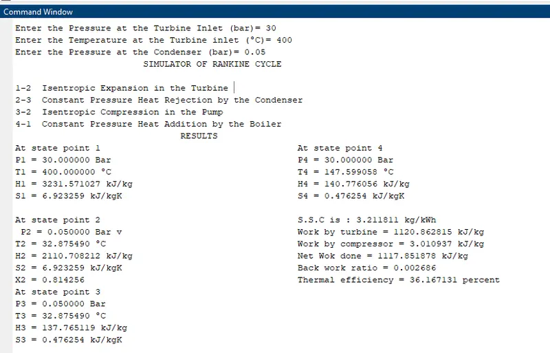
1. All State point wise values of Enthalpy, entropy,temperature.
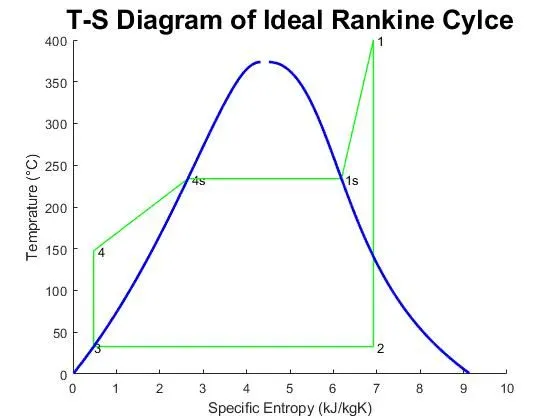
2. T-S Diagram
3.H-S Diagram
Conclusion:
from above program we calculated the work done by pump and turbine and the efficiency of the ideal rankine cycle with the help of MATLAB program.Also plotted the graph of the T-S and H-S for ideal rankine cycle.
Reference: