Week 4.1 - Genetic Algorithm

Genetic algorithm

Aim :

To make a code in Matlab to optimize the stalagmite function and to find the global maxima.

Objective :

The objective of the code is to find the global optima of the function and to explain about genetic algorithm.

Theory :

A global optimum is the extrema of the objective function for the entire input search space. Whereas a local optima is also an extrema of objective function for a given region of input space.

A local optimization algorithm should be used when you know that you are in the region of the global optima or that your objective function contains a single optima, e.g. unimodal.

A global optimization algorithm should be used when you know very little about the structure of the objective function response surface, or when you know that the function contains local optima

Genetic Algorithms(GAs) are adaptive heuristic search algorithms that belong to the larger part of evolutionary algorithms. They are commonly used to generate high-quality solutions for optimization problems and search problems.

Genetic algorithms simulate the process of natural selection which means those species who can adapt to changes in their environment are able to survive and reproduce and go to next generation.

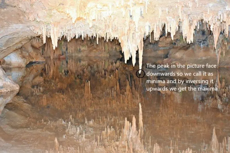
Stalagmite is a deposit of calcium carbonate like an inverted stalactite formed on the floor of a cave by the drip of calcareous water.

Calculations :

To simplify the problem we make a function stalagmite and we include the formulas inside the function to get results

function f= stalagmite(input_vector)

x = input_vector(1);

y = input_vector(2);

`f1 = (sin(5.1*pi*x+0.5)).^6`

`f2 = (sin(5.1*pi*y+0.5)).^6`

`f3 = exp((-4*log(2)*(x-0.0667).^2)/0.64)`

`f4 = exp((-4*log(2)*(y-0.0667).^2)/0.64)`

`[f] = -(f1.*f2.*f3.*f4)`

End

Genetic algorithm(‘ga’) is an in-built Matlab function which only minimizes a function. So here to maximize the function we use ( - ) of minimum values.

F(x) = - f(x)

Code presentation :

%optimization of stalagmite function using ga 
clear all
close all
clc

%defining our search space 
x = linspace(0,1,150);
y = linspace(0,1,150);
num_cases = 150;
[xx,yy] = meshgrid(x,y);
%evaluvating the stalagmite function
for i=1:length(xx)
    for j=1:length(yy)
    input_vector(1)=xx(i,j);
    input_vector(2)=yy(i,j);
    f(i,j) = stalagmite(input_vector);
    end
end

tic
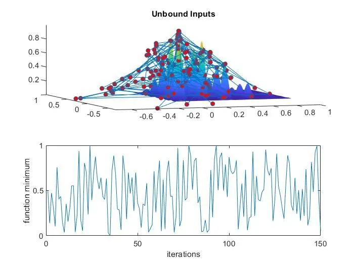
%study1-unbounded condition, statistical behaviour
for i=1:num_cases
    [inputs,fopt1(i)]=ga(@stalagmite,2);
    %ga is an inbuilt function 
    %@ defines what function to minimise
    %2 denotes the no of variables in the function, here it is x and y
    xopt(i) = inputs(1);
    yopt(i) = inputs(2);
end
study1_time = toc;
figure(1)
subplot(2,1,1)
hold on
surfc(x,y,-f)
shading interp
plot3(xopt,yopt,-fopt1,'marker','o','markersize',5,'markerfacecolor','r');
title('Unbound Inputs')
subplot(2,1,2);
plot(-fopt1);
xlabel('iterations');
ylabel('function minimum');

tic
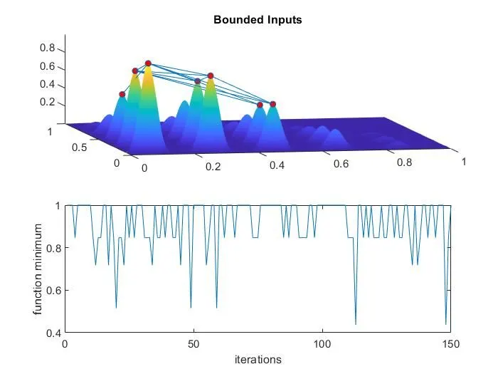
%study2-statistical behaviour(bounded), with upper and lower bounds
for i = 1:num_cases
    [inputs,fopt2(i)] = ga(@stalagmite,2,[],[],[],[],[0;0],[1;1]);
    xopt(i) = inputs(1);
    yopt(i) = inputs(2);
end
study2_time = toc;
figure(2)
subplot(2,1,1)
hold on
surfc(x,y,-f)
shading interp
plot3(xopt,yopt,-fopt2,'marker','o','markersize',5,'markerfacecolor','r');
title('Bounded Inputs')
subplot(2,1,2);
plot(-fopt2);
xlabel('iterations');
ylabel('function minimum');

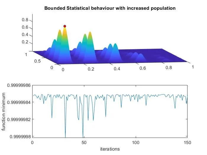
%stage3 increasing GA itrations (bounded)
options = optimoptions('ga')
options = optimoptions(options,'populationsize',500);
tic
for i = 1:num_cases
    [inputs,fopt3(i)] = ga(@stalagmite,2,[],[],[],[],[0;0],[1;1],[],[],options);
    xopt(i) = inputs(1);
    yopt(i) = inputs(2);
end
study3_time= toc;
figure(3)
subplot(2,1,1)
hold on
surfc(x,y,-f)
shading interp
plot3(xopt,yopt,-fopt3,'marker','o','markersize',5,'markerfacecolor','r');
title('Bounded Statistical behaviour with increased population')
subplot(2,1,2);
plot(-fopt3);
xlabel('iterations');
ylabel('function minimum');

fprintf ('the results are below :\n');
fprintf ('study 1 : unbounded statical behaviour\n');
fprintf ('time taken for study 1 is : %f\n',study1_time);
fprintf ('the co-ordinates of x and y for global maxima of the function are : %f,%f\n',input_vector(1),input_vector(2));
fprintf ('the global maxima of the function is : %f\n', -(mean(fopt1)));

fprintf ('study 2 : bounded statical behaviour\n');
fprintf ('time taken for study 2 is : %f\n',study2_time);
fprintf ('the co-ordinates of x and y for global maxima of the function are : %f,%f\n',input_vector(1),input_vector(2));
fprintf ('the global maxima of the function is : %f\n', -(mean(fopt2)));

fprintf ('study 3 : Bounded Statistical behaviour with increased population\n');
fprintf ('time taken for study 3 is : %f\n',study3_time);
fprintf ('the co-ordinates of x and y for global maxima of the function are : %f,%f\n',input_vector(1),input_vector(2));
fprintf ('the global maxima of the function is : %f\n', -(mean(fopt3)));

Code explanation :

Clear all, close all and clc to clear the old values and to make it as a new code.

Here the search space is defined using linspace command for both x and y variables and we fix a value for num of cases.

To make it in a 2D grid we use meshgrid (x,y) and to evaluvate the function stalagmite we use for loops (I & j).

We include tic and tok commands to get the study time for the three different optimization.

The three optimization are unbounded condition statistical behaviour, statistical behaviour with upper and lower bounds and next is increasing the ga iterations.

Plot for three studies will be between f minimum and number of iterations.

We include ‘shading interp’ command to make the figure look good without any lines and ‘surfc’ commend to generate the surface.

Result :

Stalagmite function to find the global maxima of the function is done by using Matlab and we got the results.

Conclusion :

Here we concluded the code in Matlab to optimize the stalagmite function, maxima values and the result figures of three different conditions attached below