Project 2 - Rankine cycle Simulator
Rankine cycle simulator
Aim :
To create a Rankine cycle simulator by using the xsteam data file and to make the calculations in Matlab
Objective :
The objective is to do the required Rankine cycle calculations and to plot the TS and HS diagram
Theory :
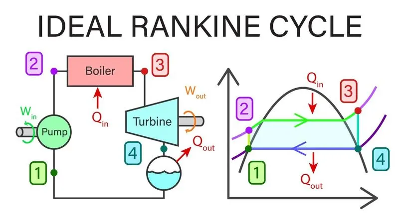
The Rankine cycle is an idealized thermodynamic cycle describing the process by which certain heat engines, such as steam turbines or reciprocating steam engines, allow mechanical work to be extracted from a fluid as it moves between a heat source and heat sink.
In this mechanism, a fuel is used to produce heat within a boiler, converting water into steam which then expands through a turbine producing useful work
A Rankine cycle power system comprises four main components: a boiler (sometimes called evaporator), a turbine, a condenser and a pump
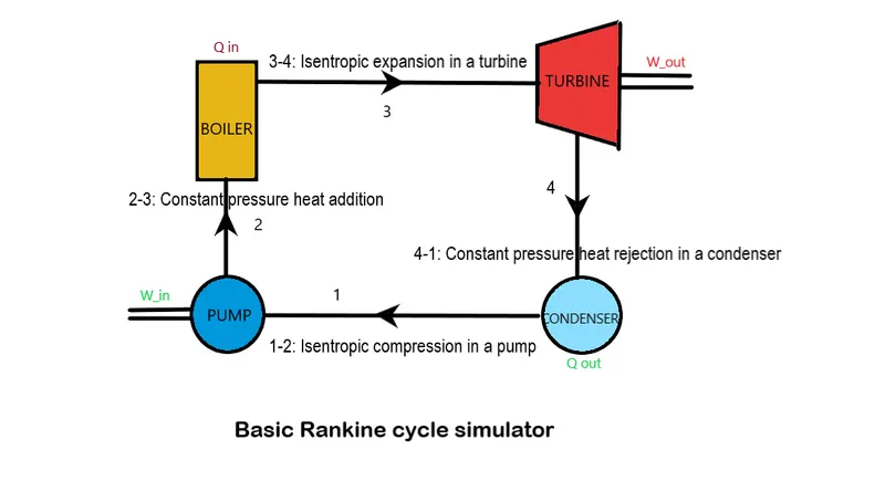
1-2: Isentropic compression in a pump.
2-3: Constant pressure heat addition in a boiler.
3-4: Isentropic expansion in a turbine.
4-1: Constant pressure heat rejection in a condenser.
Calculations :
The values that are to calculated are:
work done by turbine : wt = h1 - h2;
work done by pump : wp = (v3*(p1-p2))*100;
Net work : w_net = wt - wp;
heat into the system : Qin = h1 - h4;
heat out of the system : Qout = h2 - h3;
thermal_efficiency = (w_net/Qin)*100;
specific stream consuption : ssc = 3600/(wt - wp);
back work ratio : BW = wp / wt;
code presentation :
clear all
close all
clc

%%
disp('Rankine Cycle');
disp('1-2 Isentropic compression in a pump');
disp('2-3 Constant pressure heat addition in a boiler');
disp('3-4 Isentropic expansion in a turbine');
disp('4-1 Constant pressure heat rejection in a condenser');

%% obtaining input data
p1 = input('nValue of pressure at turbine inlet p1(in bar)=');
T1 = input('nValue of temperature at turbine inlet, T1(in degree, C)=');
p2 = input('nValue of pressure at condenser inlet p2(in bar)=');

% extracting Enthalpy and Entropy data
% state point 1
h1 = XSteam('h_pT',p1,T1);    %Enthalpy
s1 = XSteam('S_pT',p1,T1);    %Entropy

% state point 2
s2 = s1;                      %Isentropic Compression

sf2 = XSteam('SL_P',p2);      %Saturated Liquid Entropy
sg2 = XSteam('sV_P',p2);      %Saturated Vapour Entropy
hf2 = XSteam('hL_p',p2);      %Saturated Liquid Enthalpy
hg2 = XSteam('hV_p',p2);      %Saturated Vapour Enthalpy
x2 = (s2 - sf2)/(sg2 - sf2);
h2 = hf2+(x2*(hg2-hf2));

%State point 3
p3 = p2;                      %Constant Pressure Heat Addition
s3 = XSteam('sL_P',p3);
h3 = XSteam('hL_P',p3);

%State point 4
p4 = p1;
s4 = s3;

%work done by turbine
wt = h1 - h2;

%work done by pump
v3 = XSteam('vL_p',p3);
wp = (v3*(p1-p2))*100;
h4 = wp+h3;
%Net work
w_net = wt - wp;
%heat into the system
Qin = h1 - h4;
%heat out of the system
Qout = h2 - h3;
%thermal efficiency
thermal_efficiency = (w_net/Qin)*100;
%specific stream consuption : ssc = mass flow rate / power
ssc = 3600/(wt - wp);
%back work ratio
BW = wp / wt;
%calculation of temperature at state points
T3 = XSteam('Tsat_p',p3);
T2 = T3;
cp4 = XSteam('cp_ps',p4,s4);
cv4 = XSteam('cv_ps',p4,s4);
k = cp4 / cv4;
T4 = T3 / ((p3 / p4)^((k-1) / k));
%calculation of temperature, entropy and enthalpy at the vapour and liquid
%line for plotting
T6 = XSteam('tsat_p',p1);
T5 = T6;
s5 = XSteam('sL_p',p1);
s6 = XSteam('sV_p',p1);
h5 = XSteam('hL_p',p1);
h6 = XSteam('sV_p',p1);

%plotting the saturation curve
T = linspace(1,450,1000);
for i= 1:length(T)
    sf(i) = XSteam('sL_T',T(i));
    sg(i) = XSteam('sV_T',T(i));
    hf(i) = XSteam('hL_T',T(i));
    hg(i) = XSteam('hV_T',T(i));
end

% plotting T - S diagram
figure(1)
hold on
plot(sf,T,'r','LineWidth',1);
plot(sg,T,'r','LineWidth',1);
plot([s1 s2],[T1 T2],'b','LineWidth',1.5);
plot([s2 s3],[T2 T3],'b','LineWidth',1.5);
plot([s3 s4],[T3 T4],'b','LineWidth',1.5);
plot([s4 s5],[T4 T5],'b','LineWidth',1.5);
plot([s5 s6],[T5 T6],'b','LineWidth',1.5);
plot([s6 s1],[T6 T1],'b','LineWidth',1.5);
title('Temperature vs Entropy plot');
xlabel('Entropy (S) kJ/kgk')
ylabel('Temperature (degree celcius)')
legend('saturation curve')

%plotting H - S diagram
figure(2)
hold on
plot(sf,hf,'k','LineWidth',1);
plot(sg,hg,'k','LineWidth',1);
plot([s1 s2],[h1 h2],'r','LineWidth',1.5);
plot([s2 s3],[h2 h3],'r','LineWidth',1.5);
plot([s3 s4],[h3 h4],'r','LineWidth',1.5);
plot([s4 s1],[h4 h1],'r','LineWidth',1.5);
title('Enthalpy (H) vs Entropy (S)')
xlabel('Entropy (S) kJ/kgk')
ylabel('Enthalpy (H) KJ/kg')
legend('saturation curve')

%output
fprintf('At state point 1 : \n')
fprintf('p1 is %f bar\n',p1)
fprintf('T1 is %f degreecelcius\n',T1)
fprintf('h1 is %f kJ/kg\n',h1)
fprintf('s1 is %f KJ/kgk\n\n',s1)

fprintf('At state point 2 : \n')
fprintf('p2 is %f bar\n',p2)
fprintf('T2 is %f degreecelcius\n',T2)
fprintf('h2 is %f kJ/kg\n',h2)
fprintf('s2 is %f KJ/kgk\n',s2)
fprintf('x is %f \n\n',x2)

fprintf('At state point 3 : \n')
fprintf('p3 is %f bar\n',p3)
fprintf('T3 is %f degreecelcius\n',T3)
fprintf('h3 is %f kJ/kg\n',h3)
fprintf('s3 is %f KJ/kgk\n\n',s3)

fprintf('At state point 4 : \n')
fprintf('p4 is %f bar\n',p4)
fprintf('T4 is %f degreecelcius\n',T4)
fprintf('h4 is %f kJ/kg\n',h4)
fprintf('s4 is %f KJ/kgk\n\n',s4)

%printing calculated values
fprintf('work done by turbine wt = %f KJ/kg \n',wt)
fprintf('work done by pump wp = %f KJ/kg \n',wp)
fprintf('heat added in the boiler Qin = %f KJ/kg \n',Qin)
fprintf('heat rejected in the condenser Qout = %f KJ/kg \n',Qout)
fprintf('THERMAL EFFICIENCY = %f \n',thermal_efficiency)
fprintf('specific stream consuption (ssc) = %f kJ/kwh \n',ssc)
fprintf('back work ratio BW = %f',BW)
code explanation :
- clear all, close all and clc will be used to clear the older values and windows.
- with the help of xsteam.m file we can extract the stream and water properties of entropy, enthalpy at specific pressure and temperature for sat liquid, sat vapour conditions.
- The given input variables are Value of pressure at turbine inlet p1(30 bar), Value of temperature at turbine inlet T1(400 degree C), Value of pressure at condenser inlet p2(0.05 bar).
- By using the given data we have to calculate more data variables which is required for the calculation [ P,T,S,H](1,2,3,4..).
- After getting the required values the calculation part will be calculated and plots will be done.
- Here the plot figure (1) will be between Temperature (T) vs Entropy (S).
- Plot figure (2) will be between Enthalpy (H) vs Entropy(S)
- While plotting the title, label and legends are included for good picture representation.
- The results are displayed using ‘fprintf’ command in the command window.
Result :
We have created a code using Matlab to get the unknown values which is required for the calculation in different aspects as mentioned in calculation part and the results are calculated.
Net work output (turbine) = 1120.86 KJ/kg,
back work ratio = 0.03.
The output values are printed in the command window successfully.
The plot T-s and h-s created successfully.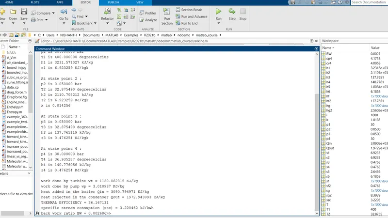
Plot presentation :
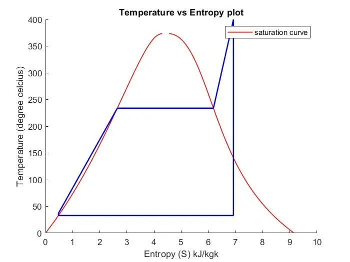
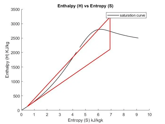
Picture with plot representation :
Conclusion :
By using the given input values we have calculated the required values and plotted it successfully.
The output values are also printed in the command window and the screenshorts are also attached for reference.
The Rankine cycle simulator is created successfully using Matlab.