Week 3 - Solving second order ODEs

Second order ordinary differential equation using Matlab

Aim:

To solve second order ordinary differential equation by using the given values through Matlab

Objective:

To make a matlab code with given values to find unknown and to plot it in a figure window

Given second order equation:

`(d^2theta) /dt^2 + b/m (d theta)/dt + g/L sintheta`

Theory:

• An ordinary differential equation(ODE) is a differential equation containing one or more functions of one independent variable and the derivatives of those functions.
• A second-order differential equation in the linear form needs two linearly independent solutions such that it obtains a solution for any initial condition, say, y(0) = a, y′(0) = b for arbitrary 'a', 'b'. In terms of mechanical perspective, the position and the velocity can be determined independently.
• PDE are very important in modelling as their solutions unlock the secrets to a range of important phenomena in engineering and physics.
• In this project we use ode45 to solve the equation and to get results
• ode45 is a six-stage, fifth-order, Runge-Kutta method.
• ode45 compares methods of orders four and five to estimate error and determine step size.
• ode45 is so accurate that its default behaviour is to use its interpolant to provide results at intermediate points.

Calculatios:

function`[(d theta)/dt]`=ode_function(t,theta,b,g,L,m)

`theta1 = theta(1)`;

`theta2 = theta(2)`;

`(d theta1)/dt = theta2`;

`(d theta2)/dt = -(b/m)*theta2 - (g/L)*sin(theta1)`;

`(d theta) /dt = [(d theta1)/dt;(d theta2)/dt]`;

end

solve ordinary differential equation

[t,results]=ode45(@(t,theta)ode_function(t,theta,b,g,l,m),t_span,theta_0);

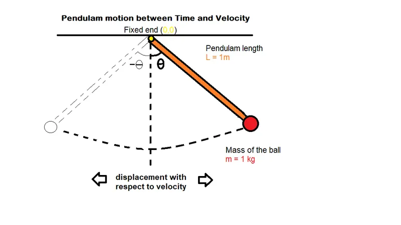
Picture representation

Matlab code:

clear all
close all
clc
%damping coefficient
b=0.05;
%gravity in m/s^2 
g=9.81;
%length of pendulam in m
L=1;
%mass of ball in kg
m=1;
%initial condition [initial displacement,initial velocity]
theta_0=[0;3];
%time points
t_span=linspace(0,20,200);
%solve ordinary differential equation
[t,results]=ode45(@(t,theta)ode_function(t,theta,b,g,L,m),t_span,theta_0);
figure(1)
plot(t,results(:,1))
hold on
plot(t,results(:,2))
ylabel('velocity');
xlabel('time in seconds');
legend('displacement','velocity');

Code explanation:

Clear all, close all and clc are used to remove old functions and values,

We take damping coefficient, gravity, length and mass as known values

And movement theta_0 will be in matrix form with initial displacement ; initial velocity [0;5].

And array of 500 values between 0 to 10 will be denoted as t_span,

The values will be taken to the above formula [t,results] to get the required unknown values by using ode_function.

[t,results]=ode45(@(t,theta)ode_function(t,theta,b,g,L,m),t_span,theta_0).

ode45 is so accurate that its default behaviour is to use its interpolant to provide results at intermediate points.

It is required to plot the output for the time 20 seconds and velocity of 3 rad/sec.

We take 200 values between 0 to 20 by using linspace command.

By appling the values in the formula [t,results] we can get the requirerd results.

The figure plot will be between time and velocity

Result:

We got the required result by placing the known values into the formula and we got the required unknown values through Matlab.­­­­­­­

Conclution:

By using Matlab we got the required values and output figure successfully.