Challenge

Week 4.1 - Genetic Algorithm

AAnandu Sasi Krishnan20 Feb 2022

AIM:

Write a code in MATLAB to optimize the stalagmite function and find the global maxima of the function.

OBJECTIVE:

Write a code in MATLAB to optimize the stalagmite function and find the global maxima of the function.
Explain the concept of genetic algorithms.
Explain the syntax for ga in MATLAB in your report.
Plot graphs for all 3 studies and for F maximum vs no. of iterations.

THEORY:

A genetic algorithm is an optimization method based on the principle of natural selection proposed by Charles Darwin. It searches for the optimal solution in the solution space. It starts with a random population of the solution and at each iteration reproduction of the new solution is done to optimize the solution.

The steps in the process of optimization through a Genetic algorithm are:

The algorithm begins by creating a random initial population.
The algorithm then creates a sequence of new populations. At each step, the algorithm uses the individuals in the current generation to create the next population. To create the new population, the algorithm performs the following steps:
1. Scores each member of the current population by computing its fitness value. These values are called the raw fitness scores.
2. Scales the raw fitness scores to convert them into a more usable range of values. These scaled values are called expectation values.
3. Selects members, called parents, based on their expectations.
4. Some of the individuals in the current population that have lower fitness are chosen as elite. These elite individuals are passed to the next population.
5. Produces children from the parents. Children are produced either by making random changes to a single parent—mutation—or by combining the vector entries of a pair of parents—crossover.
6. Replaces the current population with the children to form the next generation.
The algorithm stops when one of the stopping criteria is met.

The Matlab syntax for the genetic algorithm used is:

[x,fval] = ga(fun,nvars,A,b,Aeq,beq,lb,ub,nonlcon,intcon,options)

where

ga is the inbuilt genetic algorithm Matlab function.
x is the minimum value returned by the function.
fval is the value of the fitness function at x.
fun is the function to be minimized.
nvars is the dimensions of 'fun'.
A, b are coefficients of linear inequalities A*x ≤ b for which function is minimized.
Aeq and beq are used to find a local minimum x to fun, subject to the linear equalities Aeq*x = beq and A*x ≤ b.
lb and ub are the lower and upper bounds so that a solution is found in the range lb ≤x ≤ ub.
nonlcon is the nonlinear constrains.
intcon is a vector of positive integers taking values from 1 to nvars
options are the optimization parameters set by the user.

if there exists no inequalities A=[],b=[],Aeq=[] and beq=[].nonlcon=[] if there are no nonlinear constraints.

CODE:

FUNCTIONS:

STALAGMITE FUNCTION

function [f]=stalagmite(inputvector)
f1 = (sin(5.1*pi*inputvector(1)+0.5))^6;
f2 = (sin(5.1*pi*inputvector(2)+0.5))^6;
f3 = exp(-4*log(2)*((inputvector(1)-0.0667)^2)/(0.64)); 
f4= exp(-4*log(2)*((inputvector(2)-0.0667)^2)/(0.64)); 
f = -(f1*f2*f3*f4);
end

CODE:

clear all
close all
clc

x=linspace(0,0.6,150);                      %define a 1-D array for x
y=linspace(0,0.6,150);                      %define a 1-D array for y 
num=150;
[xx yy]=meshgrid(x,y);                      %1-D to 2-D array

for i=1:length(xx)
    for j=1:length(yy)
        inputvector(1)=xx(i,j);
        inputvector(2)=yy(i,j);
        f(i,j)=stalagmite(inputvector);    % call stalagmite function
    end
end

%unbounded
tic
for i=1:num;
    [x,fval(i)]=ga(@stalagmite,2);
    xv(i)=x(1);
    yv(i)=x(2);
end
study1=toc;
clc
figure(1)
subplot(2,1,1)
hold on
surfc(xx,yy,f)
shading interp;
plot3(xv,yv,fval,'Marker','o','MarkerSize',10,'MarkerFaceColor','r');
title('unbounded')
subplot(2,1,2)
plot(fval);
xlabel('iterations');
ylabel('function minimum');

%bounded 
tic
for i = 1:num
 [x,fval(i)] = ga(@stalagmite,2,[],[],[],[],[0,0],[1,1]);
 xv(i)=x(1);
 yv(i)=x(2);
end
study2 = toc;
clc
figure(2)
subplot(2,1,1)
hold on
surfc(xx,yy,f)
shading interp
plot3(xv,yv,fval,'Marker','o','MarkerSize',10,'MarkerFaceColor','r')
title('bounded')
subplot(2,1,2)
plot(fval)
xlabel('iterations')
ylabel('function maximum')

%optimization
options = optimoptions('ga');
options = optimoptions(options,'PopulationSize',500);
tic
for i = 1:num
 [x,fval(i)] = ga(@stalagmite,2,[],[],[],[],[0;0],[1;1],[],[],options);
 xv(i) = x(1);
 yv(i) = x(2);
end
study3 = toc;
clc
%optimisation
figure(3)
subplot(2,1,1)
hold on
surfc(xx,yy,f)
shading interp
plot3(xv,yv,fval,'Marker','o','MarkerSize',20,'MarkerFaceColor','r')
title('Optimisation with a population size of 500')
subplot(2,1,2)
plot(fval)
xlabel('iterations')
ylabel('function maximum')

clc
disp("time taken for unbounded study is "+study1);
disp("time taken for bounded study is "+study2);
disp("time taken for optimization is "+study3+"s with a population size of 500");

EXPLANATION:

FUNCTIONS:
1. STALAGMITE FUNCTION:
  - The function takes in the 'inputvector' which contains the x and y coordinate values which are to be used as inputs for the stalagmite function
    ,where f1x,f1y,f2x and f2y are defined as in the code
  - after calculating f1x,f1y,f2x, and f2y their product is returned as the result of the function.
CODE :
1. Initially, the x and y range is given as 0 to 0.6 with a range of 150, and num is given as 50.
2. We will store the x,y values in a 2d array by using meshgrid function.
3. The function which we stored is called in this code for loop function in which our inputvector is used to store x and y values into 2 columns inputvector(1) and inputvector(2).
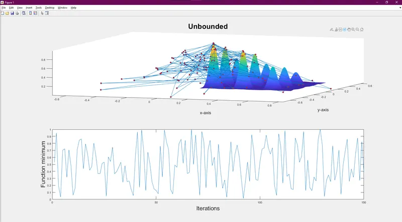
4. The study behavior for figure 1 with unbounded inputs includes calling our predefined function in a loop function and running it with our number of num.
5. The study time for 1st plot is calculated and the surface plot is employed here. The subplot defines the rows, columns, and position of the variable.
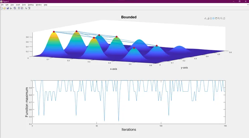
6. The study behavior for figure 2 with bounded inputs includes calling our predefined function as in study behavior 1. The only difference between 1 and 2 is, that plot 2 will have a different syntax of ga such that it will define along with the range of inputs.
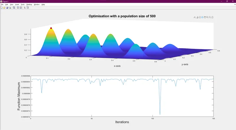
7. The study behavior for figure 3 with an increase in options includes calling predefined function as in both studies. The difference among all three studies is, in the third study we define the population size so that the number of populations in each generation is given as 500.
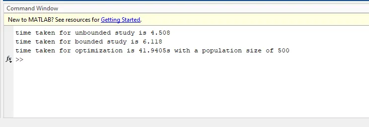
8. Thus all three figures have been obtained with the given values. and the time is taken for GA calculations for each study is displayed.