Week 3 - Solving second order ODEs

AIM: Write a program to solve a second-order differential equation for the motion of a simple pendulum with dampening.

OBJECTIVE:

1. Write a function to solve the given second-order differential equation.
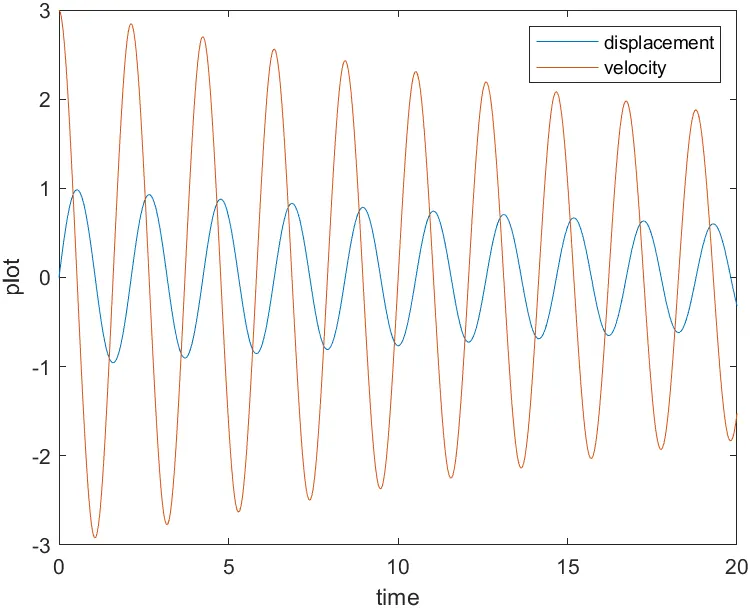
2. Plot the displacement/velocity vs time graph for the motion of the pendulum.
3. Animate the motion of the pendulum.

THEORY:

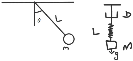
A simple pendulum consists of a small but heavy mass suspended from rigid support by a non-extensible and massless string. The rigid support is called the point of suspension, the suspended mass is considered a point mass and is usually called a bob.

This weighted mass is free to move in space when provided with an external force. When the mass is displaced sideways from its equilibrium position it is subjected to restoring force due to gravity, which tries to pull it back to the equilibrium position. This restoring force tends to oscillate the mass about its equilibrium position moving it back and forth. This motion of the pendulum will keep going until the restoring force is less than the gravity and the frictional force due to the surrounding atmosphere.

The motion of the pendulum is a circular arc. Every motion of the pendulum will make an angle with the vertical axis. This angle defines the amplitude of the oscillatory motion in the vertical plane. The greater the angle higher are the oscillations and the bigger is the arc created by the bob. We have to solve for the angle to trace the motion path of the bob, to find the change in velocity according to the time.

GOVERNING EQUATION

This is a second-order differential equation, it needs to be simplified and transformed into the first-order differential equation

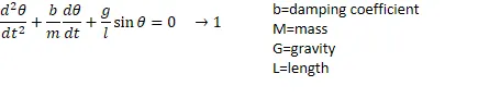
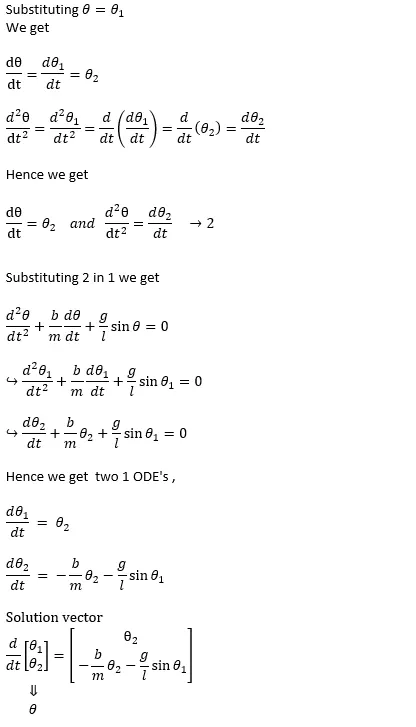
The solution vector can be used as the input function in the code, and by using the ode45 command we can compute the result by giving proper initial conditions and input parameters.

CODE:

1. FUNCTION:
   1. TO SOLVE ODE:

      function [dtheta]=ode_function(t,theta,b,g,l,m)
          theta1=theta(1);
          theta2=theta(2);
          dtheta_1=theta2;
          dtheta_2=-(b/m)*theta2-(g/l)*sin(theta1);
          dtheta=[dtheta_1;dtheta_2];
      end​

   2. TO ANIMATE THE SIMPLE PENDULUM:

      function pendulum_position(results,l)
      n=1;
      x=0;
      y=-l;
      figure (2)
      for i=1:length(results(:,1))
          theta_x=results(i,1);
          
          x=l*sin(theta_x);
          y=-l*cos(theta_x);
      
          plot([0 0],[0 -1],'LineStyle',":",'LineWidth',3,'color','k');
          hold on
          plot([0 x],[y y],'LineStyle',":",'LineWidth',3,'color','k');
          hold on
          plot([0 x],[0 y],'color','b',LineWidth=6);
          hold on
          plot([-1 1],[0 0],'LineWidth',6,'Color','k');
          hold on
          plot (x,y,'marker','o','MarkerSize',20,'MarkerFaceColor','r')
          hold off
          grid on
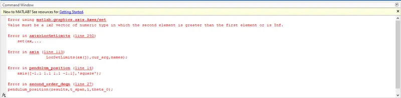
          axis([-1.1 1.1 -1.1 1.1],'square');
          pause(0.01);
          M(n)=getframe(gcf);
          n=n+1;
      end
      
      %video creation
      movie(M);
      Videofile=VideoWriter('simple_pendulum.avi','uncompressed AVI');     %creates videofile
      open(Videofile);                                                     %opens file
      writeVideo(Videofile,M);                                             %writes captured frames to file
      close(Videofile);                                                    %closes file
      
      end

2. MAIN BODY:

   clear all
   close all
   clc
   
   %inputs 
   b=0.05;                                  % damping coeeficient
   m=1;                                     % mass
   g=9.81;                                  % gravity
   l=1;                                     % length
   
   %initial condition
   theta_0=[0; 3];                          % displacement 0 and velocity 3m/s
   
   %time 
   t_span=linspace(0,20,500);
   
   %inbuilt ODE solver
   [t,results]=ode45(@(t,theta) ode_function(t,theta,b,g,l,m),t_span,theta_0);
   
   %plot time,displacement/velocity graph
   figure(1)
   plot(t,results(:,1));
   hold on
   plot(t,results(:,2));
   xlabel('time');
   ylabel('plot');
   
   pendulum_position(results,t_span,l,theta_0);​

EXPLANATION:

1. In the above code, we have created a function that solves the simplified second-order differential equation.
   • This function takes input values of mass, length, damping coefficient, initial velocity initial displacement, and time.
   • this function consists of the solution matrix of the simplified form of the second-order differential equation and calculates θ1 and θ2.
2. Another function is created to make an animation of the movement of the pendulum by plotting the position of the bob on cartesian coordinates using the values of displacement and time.
3. The main code consists of
   1. the input values and initial conditions of the pendulum
   2. an inbuilt ODE solver ode45 to get the values of displacement and velocity over a period of time
   3. code to plot velocity and displacement vs time graph

OUTPUT:

https://drive.google.com/file/d/1L2C6b121Wsx7xlbBBohcFTwmsql2_xOG/view?usp=sharing

ERRORS:

1. error in the syntax of setting axis limits
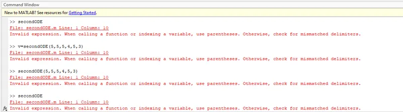
2. error in calling a function.

RESULTS:

Matlab is used to solve the given ODE and the plot of displacement/velocity vs time graph is generated and the motion of a simple pendulum is animated.