Week 4.1 - Genetic Algorithm
Write a code in MATLAB to optimise the stalagmite function and find the global maxima of the function -
Genetic Algorithm - It is a search-based optimization technique inspired by Charles Darwin's Theory of Natural Evolution. This algorithm reflects the process of natural selection where the fittest individuals are selected for reproduction in order to produce offspring of the next generation. It is used to solve non linear and non differentiable optimization problems which otherwise takes very long time to olve.
Five phases of genetic algorithm -
- Initial generation of population - The total number of candidates involved in this process is called the population and each individual is a solution. Our goal is to choose the right candidate which has the best solution for our program.
- Fitness function - This function represents how fit an individual is. This is a score by which we select the best indivual for reproduction.
- Selection - In this process we choose the parents who has good fitness function score to reproduce fittest individual for the next generation.
- Cross over - In Cross over we choose certain traits of the parents and exchange them to produce a fit child.
- Mutation - The child which has been produced, some of their genes or variables can be subjected to a mutation with a low random probability. This occurs to maintain diversity within the population.
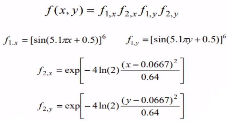
These formulas are used in the function code to generate plot in the main code.
1. Code for generating a stalagmite plot
%Defining our search space
x = linspace(0,0.6,150);
y = linspace(0,0.6,150);
[xx yy] = meshgrid(x,y);
num_cases = 50; %Number of iteration

%Evaluating the stalagmite function

for i=1:length(xx)
    for j=1:length(yy)
        input_vector(1) = xx(i,j);
        input_vector(2) = yy(i,j);
        f(i,j) = stalagmite_function(input_vector);
    end
end

surfc(xx,yy,-f);
xlabel('x value')
ylabel('y value')
shading interp
Function Code
function[f] = stalagmite_function(input_vector)

x = input_vector(1);
y = input_vector(2);

f1_x = (sin(5.1*pi*x + 0.5)).^6;
f1_y = (sin(5.1*pi*y + 0.5)).^6;

f2_x = exp((-4.*log(2))*((x - 0.0667).^2)/0.64);
f2_y = exp(-4.*log(2)*((y-0.0667).^2)/0.64);


f = -(f1_x.*f2_x.*f1_y.*f2_y);

end
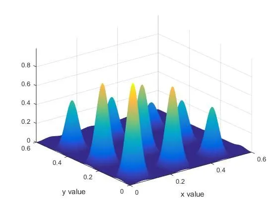
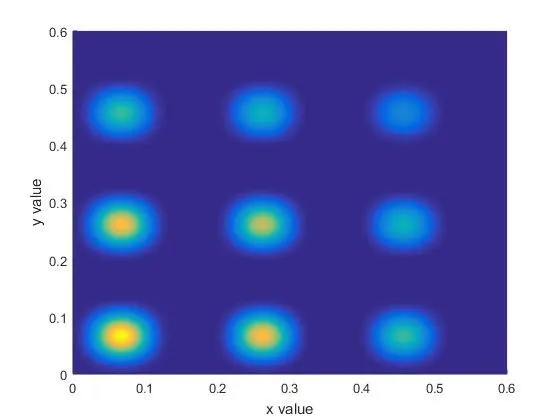
Result
Explanation
First we assign two matrices x and y then by meshgrid command we are creating another matrix [xx yy] which will be our search space. We take num_cases = 50 , this is the number of time the code will run. In the function code we take two variables x and y as input_vector(1) and input_vector(2) respectively. After calculating by using all the formulas we get the function as f = -(f1_x.*f2_x.*f1_y.*f2_y) . Now we have to run a for loop to calculate fitness function at each point in our search space. To create the stalagmite plot we are using the surfc command which will generate a 3d plot. We will take the function as negative to generate the plot upside down, this will help us to get the maxima of the function. shading interp command is use to remove the grid lines from the 3d plot.
2. First code to generate stalagmite plot for unbounded inputs
%Defining our search space
x = linspace(0,0.6,150);
y = linspace(0,0.6,150);
[xx yy] = meshgrid(x,y);
num_cases = 50; %Number of iteration

%Evaluating the stalagmite function

for i=1:length(xx)
    for j=1:length(yy)
        input_vector(1) = xx(i,j);
        input_vector(2) = yy(i,j);
        f(i,j) = stalagmite_function(input_vector);
    end
end

surfc(xx,yy,-f);
xlabel('x value')
ylabel('y value')
shading interp

%Study 1 - Statistical behavior

for i = 1:num_cases
    [inputs,fopt(i)] = ga(@stalagmite_function,2);
    xopt(i) = inputs(1);
    yopt(i) = inputs(2);

end

%Plotting
subplot(2,1,1)
surfc(xx,yy,-f);
hold on
shading interp
plot3(xopt,yopt,-fopt,'marker','o','markersize',5,'markerfacecolor','r');
title('Unbounded inputs')
xlabel('x value');
ylabel('y value');
grid on
subplot(2,1,2)
plot(-fopt);
xlabel('Iterations')
ylabel('Function minimum')
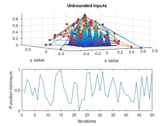
Result
Explanations
In this code the program doesnt run within a defined search space, thats why the end result is not accurate. the ga function is used to calculate the minimum value of the function we are using a negative sign to generate the plot upside down so it will give us the maxima of the function. here the syntax is ga(@stalagmite_function,2) for unbounded inputs in which @stalagmite_function calls the function code and 2 is the number of variable taken in the code.
3. Second code to generate stalagmite plot for inputs with upper and lower bounds
%Defining our search space
x = linspace(0,0.6,150);
y = linspace(0,0.6,150);
[xx yy] = meshgrid(x,y);
num_cases = 50; %Number of iteration

%Evaluating the stalagmite function

for i=1:length(xx)
    for j=1:length(yy)
        input_vector(1) = xx(i,j);
        input_vector(2) = yy(i,j);
        f(i,j) = stalagmite_function(input_vector);
    end
end

surfc(xx,yy,-f);
xlabel('x value')
ylabel('y value')
shading interp

%Study 1 - Statistical behavior

for i = 1:num_cases
    [inputs,fopt(i)] = ga(@stalagmite_function,2);
    xopt(i) = inputs(1);
    yopt(i) = inputs(2);

end

%Plotting
figure(1)
subplot(2,1,1)
surfc(xx,yy,-f);
hold on
shading interp
plot3(xopt,yopt,-fopt,'marker','o','markersize',5,'markerfacecolor','r');
title('Unbounded inputs')
xlabel('x value');
ylabel('y value');
grid on
subplot(2,1,2)
plot(-fopt);
xlabel('Iterations')
ylabel('Function minimum')


%Study 2 - Statistical behaviour with upper and lower bounds

for j = 1:num_cases
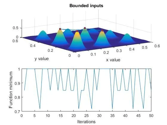
    [inputs,fopt(j)] = ga(@stalagmite_function,2,[],[],[],[],[0;0],[1;1]);
    xopt(j) = inputs(1);
    yopt(j) = inputs(2);

end

%Plotting
figure(2)
subplot(2,1,1)
surfc(xx,yy,-f);
hold on
shading interp
plot3(xopt,yopt,-fopt,'marker','o','markersize',5,'markerfacecolor','r');
title('Bounded inputs')
xlabel('x value');
ylabel('y value');
grid on
subplot(2,1,2)
plot(-fopt);
xlabel('Iterations')
ylabel('Function minimum')
Result
Explanation
In this code the program run within a defined search space, the upper and lower limits are given in function so at the end the plot is more accurate. In here the ga syntax is ga(@stalagmite_function,2,[],[],[],[],[0;0],[1;1]) in which it calls the function code first then 2 is the number of varibale taken in the code, [0;0] and [1;1] is the lower and upper bound inputs respectively.
4. Third code to generate stalagmite plot for increased population size
%Defining our search space
x = linspace(0,0.6,150);
y = linspace(0,0.6,150);
[xx yy] = meshgrid(x,y);
num_cases = 50; %Number of iteration

%Evaluating the stalagmite function

for i=1:length(xx)
    for j=1:length(yy)
        input_vector(1) = xx(i,j);
        input_vector(2) = yy(i,j);
        f(i,j) = stalagmite_function(input_vector);
    end
end

surfc(xx,yy,-f);
xlabel('x value')
ylabel('y value')
shading interp

%Study 1 - Statistical behavior

for i = 1:num_cases
    [inputs,fopt(i)] = ga(@stalagmite_function,2);
    xopt(i) = inputs(1);
    yopt(i) = inputs(2);

end


%Plotting
figure(1)
subplot(2,1,1)
surfc(xx,yy,-f);
hold on
shading interp
plot3(xopt,yopt,-fopt,'marker','o','markersize',5,'markerfacecolor','r');
title('Unbounded inputs')
xlabel('x value');
ylabel('y value');
grid on
subplot(2,1,2)
plot(-fopt);
xlabel('Iterations')
ylabel('Function minimum')


%Study 2 - Statistical behaviour with upper and lower bounds

for j = 1:num_cases
    [inputs,fopt(j)] = ga(@stalagmite_function,2,[],[],[],[],[0;0],[1;1]);
    xopt(j) = inputs(1);
    yopt(j) = inputs(2);

end


%Plotting
figure(2)
subplot(2,1,1)
hold on
surfc(xx,yy,-f);
shading interp
plot3(xopt,yopt,-fopt,'marker','o','markersize',5,'markerfacecolor','r');
title('Bounded inputs')
xlabel('x value');
ylabel('y value');
grid on
subplot(2,1,2)
plot(-fopt);
xlabel('Iterations')
ylabel('Function minimum')

%Study 3 - Increasing GA iterations
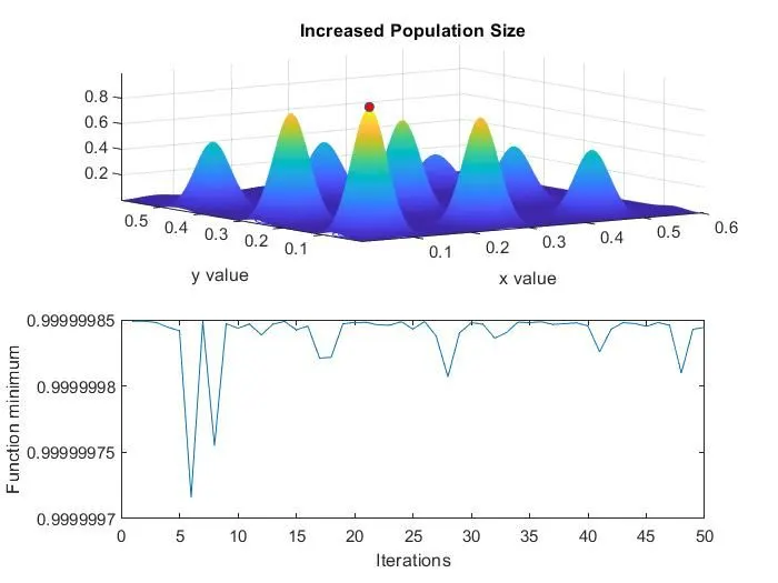
options = optimoptions('ga','populationsize',300);   %increasing the size of population

for k = 1:num_cases
    [inputs,fopt(k)] = ga(@stalagmite_function,2,[],[],[],[],[0;0],[1;1],[],[],options);
    xopt(k) = inputs(1);
    yopt(k) = inputs(2);

end

%Plotting
figure(3)
subplot(2,1,1)
hold on
surfc(xx,yy,-f);
shading interp
plot3(xopt,yopt,-fopt,'marker','o','markersize',5,'markerfacecolor','r');
title('Increased Population Size')
xlabel('x value');
ylabel('y value');
grid on
subplot(2,1,2)
plot(-fopt);
xlabel('Iterations')
ylabel('Function minimum')
Result
Explanation
In this code we are using the optimoption function to increase the population size to 300. Now we have more data to calculate the best fitness of the function. It will give us more accurate information about the global maxima. Only drawback is the simulation time will increase.
references 1. https://towardsdatascience.com/introduction-to-genetic-algorithms-including-example-code-e396e98d8bf3