Week 3 - Solving second order ODEs

Program to solve the below ODE -

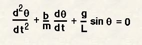* (This ODE represents the equation of motion of a simple pendulum with damping)

First Code

%Inputs
b=0.05; %Damping Coefficient
g=9.81; %Gravity in m/s^2
l=1;    %Length of the pendulum in meter
m=1;    %Mass of the ball in kg

%Initial condition
theta_0 = [0;3]; 

%Time points
t_span = linspace(0,20,500);

%Solve ODE
[t,results] = ode45(@(t,theta) function_second_order(t,theta,b,g,l,m),t_span,theta_0);

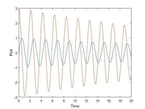
figure(1)

plot(t,results(:,1))
hold on
plot(t,results(:,2))
ylabel('Plot')
xlabel('Time')


%Animation 
displacement = results(:,1);
ct = 1;

for i = 1:length(displacement)
    THETA = displacement(i);
    x0 = 0; %Fixed point of one end of the string
    y0 = 1; %Fixed point of one end of the string
    
    x1 = 1*sin(THETA);
    y1 = -1*cos(THETA);
    
    figure(2)
    
    %Plotting
    plot([-1 1],[1 1],'linewidth',3,'color','blue'); %The pendulum is hanging by this line
    
    hold on
    
    plot([x0 x1],[y0 y1],'linewidth',2,'color','red') %String of the pendulum
    plot(x1,y1,'o','markers',20,'color','black') %Attached mass at the end of the pendulum
    
    hold off
    
    grid on
      
    axis([-2 2 -1.5 2])
    pause(0.05)
    
    M(ct) = getframe(gcf);
   
    ct = ct+1;
    
end

movie(M)
videofile = VideoWriter('pendulum_animation.avi','uncompressed AVI');
open(videofile)
writeVideo(videofile,M)
close(videofile)

Function Code

function [dtheta_dt] = function_second_order(t,theta,b,g,l,m)

theta1 = theta(1);
theta2 = theta(2);
dtheta1_dt = theta2;
dtheta2_dt = -(b/m)*theta2-(g/l)*sin(theta1);
dtheta_dt = [dtheta1_dt; dtheta2_dt];

end

Result

Pendulum Animation

https://youtu.be/MTG73B-gDEY

Explanation

The first code solves the second order differential equation and helps us to simulate a pendulum animation. First we take given inputs of damping coeffiecient, gravity, length of the string in meter, Mass of the ball attached at the end of the string. We take initial conditions which is also given , angular displacement and angular velocity. We have to simulate the pendulum in between 0 to 20 seconds so we take an array of 500 values by using the linspace command. Next to solve the ode we are using the ode45 command. In the command we have to use a function. The function code function_second_order solves the differential equation and creates a matrix dtheta_dt = [dtheta1_dt; dtheta2_dt]. Next we are plotting displacement and velocity curve in figure(1) plot window. [t,results] is a matrix so we can take the value of either displacement or velocity to plot the curves respectively. After that comes the code to simulate the animation. we are taking a displacement column from result matrix and forming a new matrix displacement = results(:,1). We have to simulate the position of the string for each value of angle THETA so we are using a for loop here. i = 1:length(displacement) means i has the value of to the number of data available in displacement matrix. so the angle THETA of the pendulum will be changing in i number of times. Now we are fixing one end of our string by assigning the values of x0 and y0. x1 and y1 is the point of the end of the string. Its changing in the loop. so x1 is x1 = 1*sin(THETA) and y1 is y1 = -1*cos(THETA). Now in the figure(2) plot window first we are plotting a line which represents a line by which the pendulum is hanging. Then hold on command to generate another plot in the same window and finally we plot the string of the pendulum by creating a line. Using marker command we create a mass attached at the end of the pendulum. We are fixing our x limit and y limit in this line axis([-2 2 -1.5 2]). We are generating a frame each in each 0.05 second. We are taking a variable M to represent each frame. now we are ending the for loop. Now we are using the movie command, we are dumping all the frames in a single .avi file called pendulum_animation. By this we are creating our animation for the pendulum motion.