Week 4.1 - Genetic Algorithm

Our task here was to understand the working of genetic algorithm solver in Matlab and use in to optimise a stalagmite function and find out the global maxima for the given funtion.

So starting with the theory behind the concept of genetic algorithm was the need to optimize an artificial function using a manmade code that was inspired by nature's way of natural selection.Now we have to figure out on how to mimic this process of natural selection into a program or an algorithm , where you give the algorithm a et of data points through which it skims and randomly selects a predefined no of these data points and then gives it to the fitness funtion(here our function to be minimised i.e. the stalagmite function) and then from the values that it gets it again modifies them through the methods of crossfiting and mutation as done in the natural selection and again feeds it into the fitness function and repeats this iterating process until and unless it arrives to a desired solution or an optimum value the defines the funtion perfectly in that search region our parameters.

How the ga() solver in Matlab works?-The Genetic Algorithm is an example of a search procedure that uses a random choice as a tool to guide a highly explorative search through a coding of a parameter space.

Working of genetic algorithm

The principle and procedure of Genetic algorithm can be summarized under the following,
1. Outline of the Algorithm.
2. Initial population.
3. Creating the Next Generation.
4. Plots of Later Generation.
5. Stopping Condition for the Algorithm.

**Let’s have a brief idea on each section.

1. Outline of the Algorithm
a. The algorithm begins by creating a random initial population.
b. The algorithm then creates a new generation or population by using the individuals of the current
population.
c. To create new generation the algorithm performs crossover and mutation in between the
individuals of the current generation.
d. Replace the current generation by the children of the next generation.
e. The children of the next generation are chosen on the basis of their best fitness value.
f. The algorithm stops when one of the stopping criteria is met.

2. Initial Population
The algorithm begins by creating a random initial population for a given problem.

Creating Next Generation: At each step, the genetic algorithm uses the current population to create the
children that makes up the next generation. The algorithm selects a group of individuals in the current
population, called ‘Parents’, who contribute their genes (The Entries Of Their Vectors) to their
children. The parents are selected on the basis of ‘Fitness’ to create better children. Genetic Algorithm
creates three types of children that are

a. Elite Children
: The individual in the current generation with best fitness value will automatically
survive to the next generation.
b.Crossover Children
: The children created by combining the genes from a pair of parents selected on
count of Fitness.
c.Mutation Children : The children created by introducing random change or mutation in the gene of a
single parent

As the number of generation increases the average fitness value of the entire generation increases and the
individuals in the population get closer to the global minimum point [0,0] of optimization.

4. Plots of Later Generation: As the algorithm goes on the graphical plot of each successive generation
shows the increasing closeness of the outcome to the global optimum point.

5.Stopping Condition for the Algorithm
The Genetic algorithm uses the following five conditions to determine when to stop.

i. Maximum Number of Generation.
ii. Maximum Time Limit.
iii. Maximum Fitness limit.
iv. Stall Generations.
v. Stall Time Limit.
The Algorithm stops as soon as any one of these five conditions met.

This is how the genetic algorithm works but what we have to note here is, the genetic algorithm will always give the local minimum value of the unconstrained function but in our task what we need is to find the global maximum so we will need to modify our ga() to give us the maximum value of the function.

Syntax

**To use the Genetic Algorithm at the command line, call the
algorithm function ’ga’ with the below mentioned syntax(This is the basic form of the syntax that we used in our program)

[x fval]=ga(@fitnessfun, nvars, options)

Where, ‘@fitnessfun’ is a handle to the Fitness Function.
‘nvars’ is the number of independent variables for the Fitness Function.
‘options’ is a structure containing options for the genetic algorithm.

The syntax returns the following things.
fval – Final Value of the Fitness Function.
X – Point at which the final value is attained.

*Now we arrive to the coding part to take a look at how this will be done.

Code and explanation

Here we divide our code into three parts that involves three studies and the stalagmite funtion code that we have to optimize.

For case 1

clear all;
close all;
clc
%Inputs or area for search
x=linspace(0,0.6,150);
y=linspace(0,0.6,150);
cases=50;
%Creating a 2D mesh
[xx, yy]=meshgrid(x,y); %This is done to provide the ga with more combination of datas to search from

%Evaluating our  satalmite function

for i=1:length(xx)
    for j=1:length(yy)
        vector(1)=xx(i,j); %Here we provide each value of the 2D array to the function using a nested for loop  
        vector(2)=yy(i,j);
        f(i,j)=stalagmite(vector); %The function returns us values or results that we store
    end
end

*Here we provide the data sets to the ga solver that are the x and y values in the form of a 2d array which will be then taken to the stalagmite function to calculate the value of function f(x,y).

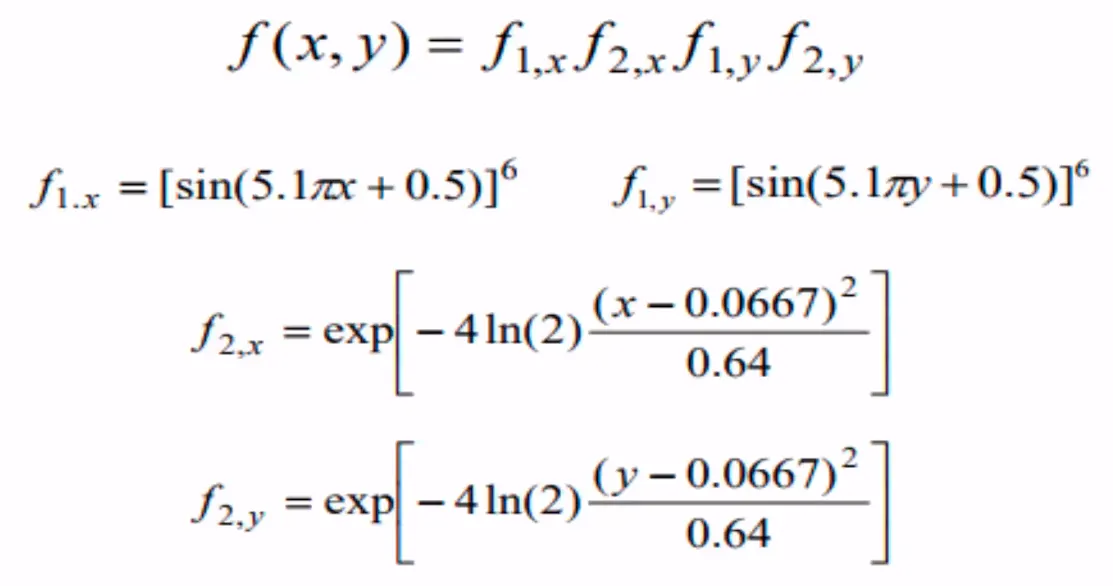
The above equation are the equations governing the stalagmite function.The code for the stalagmite function is given below.

function f=stalagmite(vector);
f1x=(sin(5.1*pi*vector(1)+0.5))^6;
f1y=(sin(5.1*pi*vector(2)+0.5))^6;
f2x=exp(-4*log(2)*((vector(1)-0.0667)^2/0.69));
f2y=exp(-4*log(2)*((vector(2)-0.0667)^2/0.69));
f=-f1x*f2x*f1y*f2y;
end

Now we move on to our first study that involves unbounded random data sets and see how ga works

%Study 1 CONSISTS OF UNBOUNDED DATA SETS
tic                                     %Timer that is used to find compilation time
for k=1:cases
    [input ,fopt(k)]=ga(@stalagmite,2); %Calling the ga solver 
    xopt(k)=input(1);                   %Storing the values of x and y for which we get the result fopt
    yopt(k)=input(2);
   
end
study_1=toc;

Here we call our ga solver and note that our ga solver is working inside a for loop so as to help ga arrive to generalized or in other words a defenite value of minimum or maximum for the function.But what happens is when we get the plots for the unbounded data sets the fopt values are scattered all around the graphs as ga doesnt know the range so it searches for a minimum from -infinity to +infinity.Now we plot the graphs for study 1.The plots have been attached with the report below.

%%The plot generation of Study 1
    figure(1)
    subplot(2,1,1)
    hold on
    surfc(xx,yy,-f)
    shading interp
    plot3(xopt,yopt,-fopt,'marker','o','MarkerSize',5,'markerfacecolor','r')
    title('Unbounded Inputs')
    subplot(2,1,2)
    plot(fopt)
    xlabel('Iterations')
    ylabel('Function maximum')
    hold off

Now we move on to our second study where we provide bounds to the data set as upper and lower bounds so as to specify the search space for the ga solver where move the search range from infinity to a certain value.

%%Same is done for study 2 ,only the upper and lower bounds are included
    %Study 2 providing the upper and lower bounds
tic;

for i=1:cases
    [input, fopt(i)]=ga(@stalagmite,2,[],[],[],[],[0;0],[0.6;0.6]);  %The syntax for ga here is different as it contains bounds
    xopt(i)=input(1);
    yopt(i)=input(2);
end
study_2=toc;
%%Generating plots for study 2
    figure(2)
    subplot(2,1,1)
    hold on
    surfc(xx,yy,-f)
    shading interp
    plot3(xopt,yopt,-fopt,'marker','o','MarkerSize',5,'markerfacecolor','r')
    title('Bounded Inputs')
    subplot(2,1,2)
    plot(fopt)
    xlabel('Iterations')
    ylabel('Function maximum')
    hold off

Here the syntax for the ga solver is changed so as to include the upper and lower bounds.The squre brackets are there for depicting other unused parameters that have not been given any values.

[input, fopt(i)]=ga(@stalagmite,2,[],[],[],[],[0;0],[0.6;0.6]);

Again we plot the graphs for the second study and find that the solution now become more clearer and concise.lying between the three peaks of minimas.

%%Generating plots for study 2
    figure(2)
    subplot(2,1,1)
    hold on
    surfc(xx,yy,-f)
    shading interp
    plot3(xopt,yopt,-fopt,'marker','o','MarkerSize',5,'markerfacecolor','r')
    title('Bounded Inputs')
    subplot(2,1,2)
    plot(fopt)
    xlabel('Iterations')
    ylabel('Function maximum')
    hold off

Now we move on to study 3.Here we provide another modyfication in ga as we increase the population size what the ga takes in.The ga solver by default takes in 50 random x-y points and then works on it again every time till the iteration are completed.Here we increase the population range from 50 to 170 so as to find out the optimum value for the function.And then plot the graphs for the study three here we cand find that the plot becomes more consie and the maximum value is not changing but is rather lying on a single peak. That maximum value of the function can be found out by studying the third study plot which is 1.The plots of the mentioned case has also been attached below the report.The maximum value of the funtion here doesnt change even after several iteration that tells us that the ga solver has arrived to a distinct value that doesnt change drastically with repeatedly excuting the loop again.

% Study 3 in case of modified population values
options=optimoptions('ga');    %Here the population size is increased
options=optimoptions(options,'PopulationSize',170);
tic;
for i=1:cases
    [input, fopt(i)]=ga(@stalagmite,2,[],[],[],[],[0;0],[0.6;0.6],[],[],options);%Another change in the syntax
    xopt(i)=input(1);
    yopt(i)=input(2);
end
%%Generating plots for study three
study_3=toc;
    figure(3)
    subplot(2,1,1)
    hold on
    surfc(xx,yy,-f)
    shading interp
    plot3(xopt,yopt,-fopt,'marker','o','MarkerSize',5,'markerfacecolor','r')
    title('Bounded Inputs with modified population size')
    subplot(2,1,2)
    plot(fopt)
    xlabel('Iterations')
    ylabel('Function maximum')
    hold off

So this was how we optimized the given stalagmite funtion using the ga solver in matlab.The complete program code is given below.

clear all;
close all;
clc
%Inputs or area for search
x=linspace(0,0.6,150);
y=linspace(0,0.6,150);
cases=50;
%Creating a 2D mesh
[xx, yy]=meshgrid(x,y); %This is done to provide the ga with more combination of datas to search from

%Evaluating our  satalmite function

for i=1:length(xx)
    for j=1:length(yy)
        vector(1)=xx(i,j); %Here we provide each value of the 2D array to the function using a nested for loop  
        vector(2)=yy(i,j);
        f(i,j)=stalagmite(vector); %The function returns us values or results that we store
    end
end

%Study 1 CONSISTS OF UNBOUNDED DATA SETS
tic                                     %Timer that is used to find compilation time
for k=1:cases
    [input ,fopt(k)]=ga(@stalagmite,2); %Calling the ga solver 
    xopt(k)=input(1);                   %Storing the values of x and y for which we get the result fopt
    yopt(k)=input(2);
   
end
study_1=toc;
%%The plot generation of Study 1
    figure(1)
    subplot(2,1,1)
    hold on
    surfc(xx,yy,-f)
    shading interp
    plot3(xopt,yopt,-fopt,'marker','o','MarkerSize',5,'markerfacecolor','r')
    title('Unbounded Inputs')
    subplot(2,1,2)
    plot(fopt)
    xlabel('Iterations')
    ylabel('Function maximum')
    hold off
%%Same is done for study 2 ,only the upper and lower bounds are included
    %Study 2 providing the upper and lower bounds
tic;

for i=1:cases
    [input, fopt(i)]=ga(@stalagmite,2,[],[],[],[],[0;0],[0.6;0.6]);  %The syntax for ga here is different as it contains bounds
    xopt(i)=input(1);
    yopt(i)=input(2);
end
study_2=toc;
%%Generating plots for study 2
    figure(2)
    subplot(2,1,1)
    hold on
    surfc(xx,yy,-f)
    shading interp
    plot3(xopt,yopt,-fopt,'marker','o','MarkerSize',5,'markerfacecolor','r')
    title('Bounded Inputs')
    subplot(2,1,2)
    plot(fopt)
    xlabel('Iterations')
    ylabel('Function maximum')
    hold off

% Study 3 in case of modified population values
options=optimoptions('ga');    %Here the population size is increased
options=optimoptions(options,'PopulationSize',170);
tic;
for i=1:cases
    [input, fopt(i)]=ga(@stalagmite,2,[],[],[],[],[0;0],[0.6;0.6],[],[],options);%Another change in the syntax
    xopt(i)=input(1);
    yopt(i)=input(2);
end
%%Generating plots for study three
study_3=toc;
    figure(3)
    subplot(2,1,1)
    hold on
    surfc(xx,yy,-f)
    shading interp
    plot3(xopt,yopt,-fopt,'marker','o','MarkerSize',5,'markerfacecolor','r')
    title('Bounded Inputs with modified population size')
    subplot(2,1,2)
    plot(fopt)
    xlabel('Iterations')
    ylabel('Function maximum')
    hold off