Week 4.1 - Genetic Algorithm

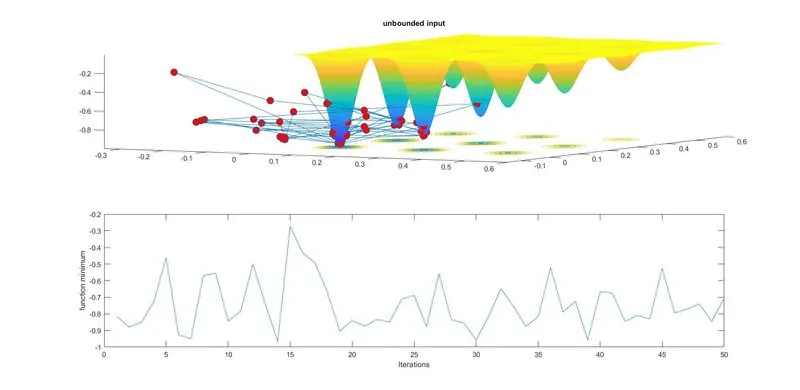
Aim: To optimize the stalagmite function and find the global maxima of the function.

Description:

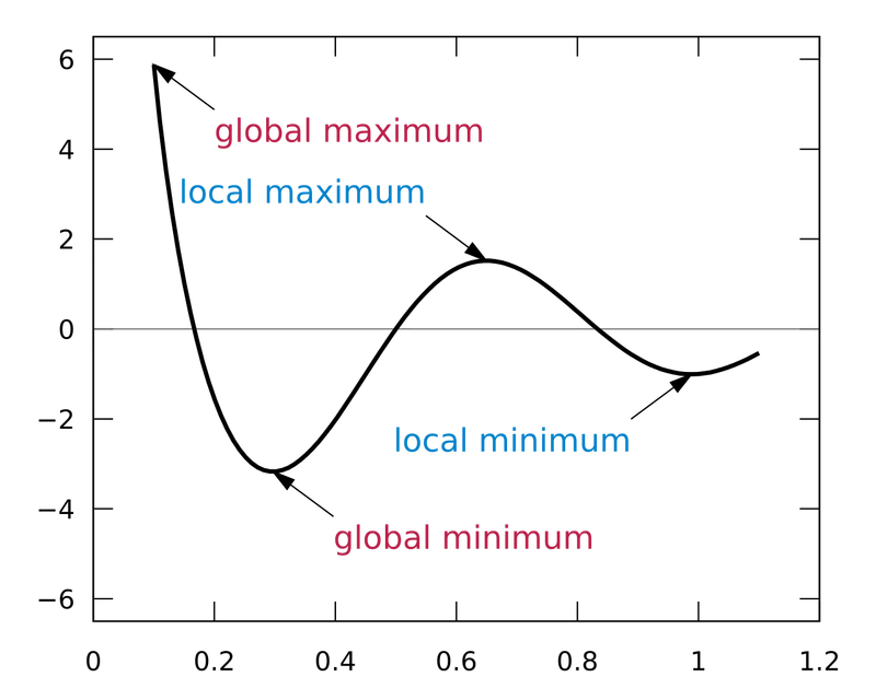
Global maxima are the highest point of a data set and are a unique point, so for a given data there can be only one global maxima, also known as an absolute maximum, the largest overall value of a set, function, etc., over its entire range. It is impossible to construct an algorithm that will find a global maximum for an arbitrary function.

A genetic algorithm (GA) is a method for solving both constrained and unconstrained optimization problems based on a natural selection process that mimics biological evolution.

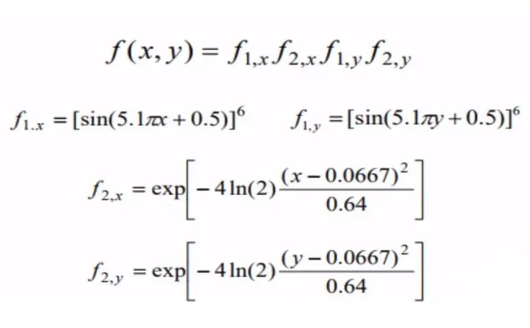
A stalagmite function generally refers to the function with which we are generating values over a stalagmite kind of surface for finding out the local and global maxima and minima of that particularly given function.

Code:

code for the stalagmite function:

function [F]= stalagmite(zz)
x=zz(1)
y=zz(2)
f1_x=(sin((5.1*pi*x)+0.5)).^6;
f1_y=(sin((5.1*pi*y)+0.5)).^6;
f2_x=exp(-4*log(2)*((x-0.0667).^2)/0.64);
f2_y=exp(-4*log(2)*((y-0.0667).^2)/0.64);
[F]=-(f1_x.*f1_y.*f2_x.*f2_y);
end

code :

x= linspace(0,0.6,150);
y= linspace(0,0.6,150);

[xx,yy]= meshgrid(x,y)

for i= 1:length(xx)
    for j= 1:length(yy)
        input_vector(1)=xx(i,j);
        input_vector(2)=yy(i,j);
        f(i,j)= stalagmite(input_vector);
    end
end

num_cases=50
tic
% study 1 
for i=1:num_cases
    [inputs,fopt(i)]=ga(@stalagmite,30);
    xopt(i)=inputs(1);
    yopt(i)=inputs(2);
end
study1_time= toc

figure(1)
subplot(2,1,1)
hold on
surfc(x,y,f)
shading interp
plot3(xopt,yopt,fopt,'marker','o','markersize',10,'markerfacecolor','r')
title('unbounded input')
subplot(2,1,2)
plot(fopt)
xlabel('Iterations')
ylabel('function minimum')


% study 2 

options=optimoptions('ga')
options=optimoptions(options,'populationsize',100)
tic
for i=1:num_cases
    [inputs,fopt(i)]=ga(@stalagmite,2,[],[],[],[],[0;0],[0.1;0.1]);
    xopt(i)=inputs(1);
    yopt(i)=inputs(2);
end
study2_time= toc

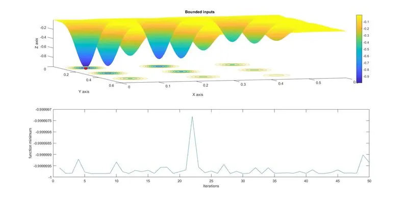
figure(2)
subplot(2,1,1)
hold on
surfc(x,y,f)
shading interp
title('Bounded inputs')
xlabel('X axis')
ylabel('Y axis')
zlabel('Z axis')
colorbar
plot3(xopt,yopt,fopt,'marker','o','markersize',10,'markerfacecolor','r')
subplot(2,1,2)
plot(fopt)
xlabel('Iterations')
ylabel('function minimum')

% study 3 
options=optimoptions('ga')
options=optimoptions(options,'populationsize',150)

tic

for i=1:num_cases
    [inputs,fopt(i)]=ga(@stalagmite,2,[],[],[],[],[0;0],[0.1;0.1],[],[],options);
    xopt(i)=inputs(1);
    yopt(i)=inputs(2);
end
study3_time= toc

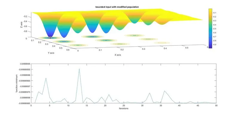
figure(3)
subplot(2,1,1)
hold on
surfc(x,y,f)
shading interp
title('bounded input with modified population')
xlabel('X axis')
ylabel('Y axis')
zlabel('Z axis')
colorbar
plot3(xopt,yopt,fopt,'marker','o','markersize',5,'markerfacecolor','r')
subplot(2,1,2)
plot(fopt)
xlabel('Iterations')
ylabel('function minimum')

Explanation:

We assume the no of cases to be 50

The tic function records the current time, and the toc function uses the recorded value to calculate elapsed time.

Interpolation (interp) is a technique for adding new data points within a range of a set of known data points.

surf() is used to create a 3d surface plot

plot3() is used to create coordinates in 3d space

subplot( m, n, p ) divides the current figure into an m -by- n grid and creates axes in the position specified by p

Results: