Project 2 - Rankine cycle Simulator

Objective:

• To create a Rankine cycle and calculate state points using the input data
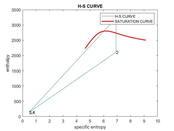
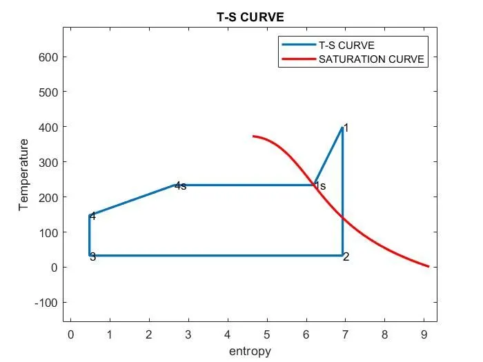
• To plot T_S and H_S for the given inputs

Description:

The Rankine cycle is an idealized thermodynamic cycle describing the process by which certain heat engines, such as steam turbines or reciprocating steam engines, allow mechanical work to be extracted from a fluid as it moves between a heat source and heat sink.

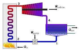
1-2: Isentropic compression in a pump.

2-3: Constant pressure heat addition in a boiler.

3-4: Isentropic expansion in a turbine.

4-1: Constant pressure heat rejection in a condenser.

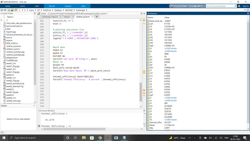
code:

clc
close all
clear all
%inputs
p1=input('pressure at intel of turbine is : ');
t1=input('temperature at the inlet of turbine: ');
p2=input('pressure at inlet of condenser: ');
%cp at p1
cp1=XSteam('cpL_p',p1);

%at point 1
disp('variables at state point 1: ')
fprintf('p1 :%f barn ',p1)
t1s=XSteam('Tsat_p',p1);
s1s=XSteam('sV_p',p1);
s1f=XSteam('sL_p',p1);
h1=XSteam('h_pT',p1,t1);
fprintf('h1 : %f KJ/Kg n',h1)
s1=XSteam('s_pT',p1,t1);
fprintf('s1 : %f KJ/Kgk n',s1)
fprintf('t1 : %f Deg celcius n',t1)

% at point 2
disp('variables at state point 2: ')
fprintf('p2 :%f barn ',p2)
s2=s1;
hg2=XSteam('hV_p',p2);
hf2=XSteam('hL_p',p2);
sg2=XSteam('sV_p',p2);
sf2=XSteam('sL_p',p2);
x2=(s2-sf2)/(sg2-sf2);
h2=hf2+x2*(hg2-hf2);
fprintf('h2 : %f KJ/Kg n',h2)
t2=XSteam('Tsat_p',p2);
fprintf('s2 : %f KJ/Kgk n',s2)
fprintf('t2 : %f Deg celcius n',t2)

% atpoint 3
disp('variables at state point 3: ')
p3=p2;
fprintf('p3 : %f bar n',p3)
hf3=XSteam('hL_p',p3);
h3=hf3;
fprintf('h3 : %f KJ/Kg n',h3)
sf3=XSteam('sL_p',p3);
s3=sf3;
fprintf('s3 : %f KJ/Kgk n',s3)
t3=t2;
fprintf('t3 : %f Deg celcius n',t3)

%at point 4
disp('variables at state point 4: ')
p4=p1;
fprintf('p4 : %f bar n',p4)
s4=s3;
hf4=XSteam('h_ps',p4,s4);
h4=hf4;
fprintf('h4 : %f KJ/Kg n',h4)
fprintf('s4 : %f KJ/Kgk n',s4)
t4=t1s/exp((s1f-s4)/cp1);
fprintf('t4 : %f Deg celcius n',t4)

t5=t1s;
s5=XSteam('sL_T',t5);

%plot
figure(1)
plot([s1 s2 s3 s4 s1],[h1 h2 h3 h4 h1])
xlabel('specific entropy')
ylabel('enthalpy')
title('H-S CURVE')
text(s1,h1,'1')
text(s2,h2,'2')
text([s3 s4],[h3 h4],'3,4')
hold on

%saturation line
TC=(1:2000);
for i=1:1:2000
    hl(i)=XSteam('hL_T',TC(i));
     sl(i)=XSteam('sL_T',TC(i));
    %saturated vapour line
     hv(i)=XSteam('hV_T',TC(i));
     sv(i)=XSteam('sV_T',TC(i));
end
% plotting saturation line
plot(s1,h1,'r','LineWidth',2)
plot(sv,hv,'r','LineWidth',2)
legend('H-S CURVE','SATURATION CURVE')

figure(2)
plot([s1 s2 s3 s4 s1f s1s s1],[t1 t2 t3 t4 t5 t1s t1],'LineWidth',2)
xlabel('entropy')
ylabel('Temperature')
text(s1,t1,'1')
text(s2,t2,'2')
text(s3,t3,'3')
text(s4,t4,'4')
text(s1s,t1s,'1s')
title('T-S CURVE')
text(s1f,t5,'4s')
hold on

% plotting saturation line
plot(s1,TC,'r','LineWidth',2)
plot(sv,TC,'r','LineWidth',2)
legend('T-S CURVE','SATURATION CURVE')
 

%work done
Wt=h1-h2
Wp=h4-h3
Wnet=Wt-Wp
fprintf('net work: %f KJ/Kg n', Wnet)
%heat in
Qin=h1-h4
Back_work_ratio=-Wp/Wt
fprintf('Back Work Ratio: %f n',Back_work_ratio)

thermal_efficiency= (Wnet*100)/Qin
fprintf('Thermal Efficiency : % percent ',thermal_efficiency)

Explanation:

Here the inputs given are:

Turbine inlet pressure= 30 bars

turbine intel temperature= 400°C

condenser inlet pressure= 0.05 Bars

Here

1-2 is an isoentropic process so s1=s2

2-3 is an isobaric process so p2=p3

3-4 is an isentropic process so s3=s4

4-1 is an isobaric process so p4=p1

h= enthalpy KJ/Kg

s= entropy KJ/Kg C

t= temperature ° C

p= pressure Bar

we calculates the required output properties

• work done
  Wt=h1-h2
  Wp=h4-h3
  Wnet=Wt-Wp
• heat input
  Qin=h1-h4
• Back_work_ratio=-Wp/Wt
• thermal_efficiency= (Wnet*100)/Qin

Plots:

Output:

pressure at intel of turbine is : 30
temperature at the inlet of turbine: 400
pressure at inlet of condenser: 0.05
variables at state point 1: 
p1 :30.000000 barn h1 : 3231.571027 KJ/Kg ns1 : 6.923259 KJ/Kgk nt1 : 400.000000 Deg celcius nvariables at state point 2: 
p2 :0.050000 barn h2 : 2110.708212 KJ/Kg ns2 : 6.923259 KJ/Kgk nt2 : 32.875490 Deg celcius nvariables at state point 3: 
p3 : 0.050000 bar nh3 : 137.765119 KJ/Kg ns3 : 0.476254 KJ/Kgk nt3 : 32.875490 Deg celcius nvariables at state point 4: 
p4 : 30.000000 bar nh4 : 140.762226 KJ/Kg ns4 : 0.476254 KJ/Kgk nt4 : 147.599058 Deg celcius n
Wt =

   1.1209e+03


Wp =

    2.9971


Wnet =

   1.1179e+03

net work: 1117.865709 KJ/Kg n
Qin =

   3.0908e+03


Back_work_ratio =

   -0.0027

Back Work Ratio: -0.002674 n
thermal_efficiency =

   36.1674