Week 4.1 - Genetic Algorithm
% MATLAB Code to optimise the stalagmite function and find the global
% maxima of the function.

% Stalagmite function
function[z] = stalagmite(input_vector)

% Defining Objective Function
x = input_vector(1); % defining inputs x
y = input_vector(2); % defining inputs y

% Formula
% z = -(f1x*f2x*f1y*f2y);

% Calculating values of input
% f1x = [sin(5.1*pi*x+0.5)].^6
% f1y = [sin(5.1*pi*y+0.5)].^6
% f2x = exp[-4ln(2).*((x-0.667).^2)./0.64]
% f2y = exp[-4ln(2).*((y-0.667).^2)./0.64]

f1x = (sin((5.1*pi*x)+0.5)).^6;
f1y = (sin((5.1*pi*y)+0.5)).^6;
f2x = exp(-4*log(2).*((x-0.667).^2)./0.64);
f2y = exp(-4*log(2).*((y-0.667).^2)./0.64);

z = -(f1x*f2x*f1y*f2y);
end


% Main Program


% Clearing Workspace, Command Window and Closing Previous Plots
clear all
close all
clc

% Inputs
x = linspace(0,0.6,150); % There 150 values between 0 to 0.6
y = linspace(0,0.6,150); % There 150 values between 0 to 0.6
num_cases = 50; % No. of iterations to 50
% Forming 2D arrays
[xx yy] = meshgrid(x,y);

for i = 1:length(xx)
    for j = 1:length(yy)
        input_vector(1) = xx(i,j);
        input_vector(2) = yy(i,j);
        f(i,j) = stalagmite(input_vector);
    end
end
tic
% Study 1 - Statistical Behavior of Unbounded Inputs

for i = 1:num_cases
    [results, fopt(i)] = ga(@ stalagmite, 2)
    xopt(i) = results(1);
    yopt(i) = results(2);
end

study1_time = toc

figure(1)
subplot(2,1,1)
surf(x, y, -f) % to get 3D surface
shading interp
hold on
plot3(xopt,yopt,-fopt,'marker','o','markersize',5,'markerfacecolor','r')
title('Unbounded Inputs')
subplot(2,1,2)
plot(-fopt)
title('Iteration vs Function Maximum')
xlabel('Iterations')
ylabel('Function minimum')

% Study 2- Statistical Behavior of Bounded Inputs

tic
for i = 1:num_cases
    [results,fopt(i)] = ga(@stalagmite,2,[],[],[],[],[0;0],[0.6;0.6]);
        xopt(i) = results(1)
        yopt(i) = results(2)
end
study2_time = toc
figure(2)
subplot(2,1,1)
surf(x,y,-f)
shading interp
hold on
plot3(xopt,yopt,-fopt,'marker','o','markersize',5,'markerfacecolor','r')
title('Bounded Inputs')
subplot(2,1,2)
plot(-fopt)
title('Iteration vs Function Maximum')
xlabel('Iteration')
ylabel('Function Maximum')

% Study 3- Statistical Behavior of Increased Initial Population
tic
options = optimoptions('ga');
options = optimoptions(options,'populationsize',250);
for i = 1:num_cases
    [results,fopt(i)] = ga(@stalagmite,2,[],[],[],[],[0;0],[0.6;0.6],[],[],options);
     xopt(i) = results(1);
     yopt(i) = results(2);
end
study3_time = toc
figure(3)
subplot(2,1,1)
surf(x,y,-f)
shading interp
hold on
plot3(xopt,yopt,-fopt,'marker','o','markersize',5,'markerfacecolor','r')
title('Increased Initial Population')
subplot(2,1,2)
plot(-fopt)
title('Iteration vs Function Maximum')
xlabel('Iteration')
ylabel('Function Maximum')
Q1. Concept of Genetic Algorithm?
Ans.
Genetic Algorithms(GAs) are versatile heuristic hunt calculations that have a place with the bigger piece of transformative calculations. Genetic algorithms depend on the thoughts of regular determination and hereditary qualities. These are shrewd double-dealing of irregular inquiry furnished with authentic information to coordinate the hunt into the locale of better execution in arrangement space. They are generally used to produce great answers for enhancement issues and search issues.
Genetic algorithms reenact the course of normal determination which implies those species who can adjust to changes in their current circumstance can get by and imitate and go to future. In basic words, they recreate "natural selection" among individual of sequential age for tackling an issue. Every age comprise of a populace of people and every individual addresses a point in search space and conceivable arrangement. Every individual is addressed as a line of character/whole number/float/bits. This string is practically equivalent to the Chromosome.
Q2. Syntax for GA?
Ans.
x = ga(fun,nvars)
finds a local unconstrained minimum, x, to the objective function,
fun. nvars is the dimension (number of design variables) of fun.
x = ga(fun,nvars,A,b)
finds a local minimum x to fun, subject to the linear inequalities
A*x ≤ b. ga evaluates the matrix product A*x as if x is transposed (A*x').
x = ga(fun,nvars,A,b,Aeq,beq)
finds a local minimum x to fun, subject to the linear equalities
Aeq*x = beq and A*x ≤ b. (Set A=[] and b=[] if no linear inequalities
exist.) ga evaluates the matrix product Aeq*x as if x is transposed
(Aeq*x').
x = ga(fun,nvars,A,b,Aeq,beq,lb,ub)
defines a set of lower and upper bounds on the design variables, x, so that
a solution is found in the range lb ≤ x ≤ ub. (Set Aeq=[] and beq=[] if
no linear equalities exist.)
x = ga(fun,nvars,A,b,Aeq,beq,lb,ub,nonlcon)
subjects the minimization to the constraints defined in nonlcon. The
function nonlcon accepts x and returns vectors C and Ceq, representing the
nonlinear inequalities and equalities respectively. ga minimizes the fun
such that C(x) ≤ 0 and Ceq(x) = 0. (Set lb=[] and ub=[] if no bounds exist.)
x = ga(fun,nvars,A,b,Aeq,beq,lb,ub,nonlcon,options)
minimizes with the default optimization parameters replaced by values in
options. (Set nonlcon=[] if no nonlinear constraints exist.) Create options
using optimoptions.
x = ga(fun,nvars,A,b,Aeq,beq,lb,ub,nonlcon,intcon) OR
x = ga(fun,nvars,A,b,Aeq,beq,lb,ub,nonlcon,intcon,options)
requires that the variables listed in intcon take integer values.
x = ga(problem)
finds the minimum for problem, a structure described in problem.
[x,fval] = ga(___)
for any previous input arguments, also returns fval, the value of the
fitness function at x.
[x,fval,exitflag,output] = ga(___)
also returns exitflag, an integer identifying the reason the algorithm
terminated, and output, a structure that contains output from each
generation and other information about the performance of the algorithm.
[x,fval,exitflag,output,population,scores] = ga(___)
also returns a matrix population, whose rows are the final population,
and a vector scores, the scores of the final population.
Q3. Detailed explanation of the program?
Ans.
Explanation of the program including the stalagmite function
Study 1 : Unbounded Values
Step - 1 - Giving 2 inputs x & y taking 150 values between 0 to 0.6.
x = linspace(0,0.6,150); % There 150 values between 0 to 0.6
y = linspace(0,0.6,150); % There 150 values between 0 to 0.6
num_cases = 50; % No. of iterations to 50
Step - 2 - Form 2D arrays for the 'x' & 'y' inputs
[xx yy] = meshgrid(x,y);
Step - 3 - Stalagmite function is used to plot a 3D surface plot using
the new 'XX' & 'YY' 2D arrays which is stored in 'input_vector'.
for i = 1:length(xx)
for j = 1:length(yy)
input_vector(1) = xx(i,j);
input_vector(2) = yy(i,j);
f(i,j) = stalagmite(input_vector);
end
end
Step - 4 - Here, the stalagmite function gives the output as (-f) which
is the maxima, since 'ga' only minimizes the function.
% Stalagmite function
function[z] = stalagmite(input_vector)
% Defining Objective Function
x = input_vector(1); % defining inputs x
y = input_vector(2); % defining inputs y
% Formula
% z = -(f1x*f2x*f1y*f2y);
% Calculating values of input
% f1x = [sin(5.1*pi*x+0.5)].^6
% f1y = [sin(5.1*pi*y+0.5)].^6
% f2x = exp[-4ln(2).*((x-0.667).^2)./0.64]
% f2y = exp[-4ln(2).*((y-0.667).^2)./0.64]
f1x = (sin((5.1*pi*x)+0.5)).^6;
f1y = (sin((5.1*pi*y)+0.5)).^6;
f2x = exp(-4*log(2).*((x-0.667).^2)./0.64);
f2y = exp(-4*log(2).*((y-0.667).^2)./0.64);
z = -(f1x*f2x*f1y*f2y);
end
Step - 5 - Using the iteration loop for 'ga' to calculate the maxima
of the function. Outputs are stored in 'results' that contain
maxima and 'fopt' contains the value at which the maxima is
obtained
tic
% Study 1 - Statistical Behavior of Unbounded Inputs
'ga' is initiated with a random population
for i = 1:num_cases
[results, fopt(i)] = ga(@ stalagmite, 2)
xopt(i) = results(1);
yopt(i) = results(2);
end
In order to get the complete cycle, 'tic' 'toc' command is used to record
time
study1_time = toc
figure(1)
subplot(2,1,1)
surf(x, y, -f) % obtaining 3D surface
shading interp
hold on
plot3(xopt,yopt,-fopt,'marker','o','markersize',5,'markerfacecolor','r')
title('Unbounded Inputs')
subplot(2,1,2)
plot(-fopt)
title('Iteration vs Function Maximum')
xlabel('Iterations')
ylabel('Function minimum')
Storing the results into xopt,yopt, plot the surface of x,y,-f to get the
3D plot
Study - 1 - Output >>>>
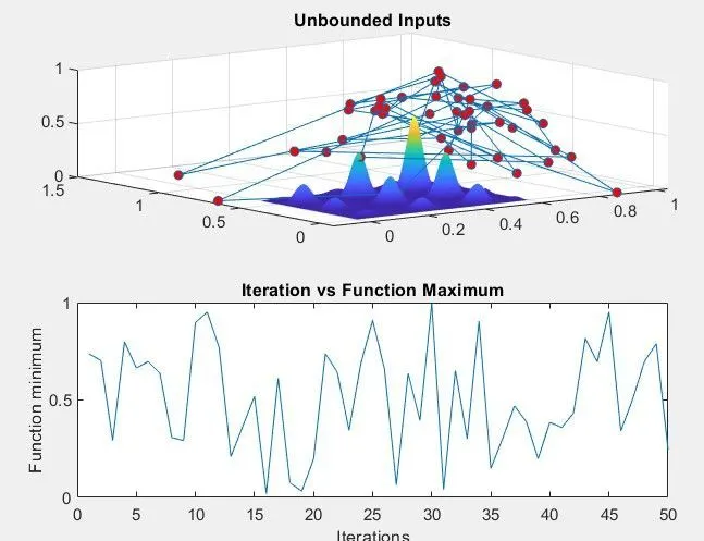
The optimal values went outside the range of 'x' and 'y' values that
drifted away from the stalgamite surface, failing to obtain maxima
Elapsed study time = 3.4044
Study - 2 - Bonded Values
Specifying the range of x and y , the 'ga'is initiated with a
random population only.
tic
for i = 1:num_cases
[results,fopt(i)] = ga(@stalagmite,2,[],[],[],[],[0;0],[0.6;0.6]);
xopt(i) = results(1)
yopt(i) = results(2)
end
study2_time = toc
figure(2)
subplot(2,1,1)
surf(x,y,-f)
shading interp
hold on
plot3(xopt,yopt,-fopt,'marker','o','markersize',5,'markerfacecolor','r')
title('Bounded Inputs')
subplot(2,1,2)
plot(-fopt)
title('Iteration vs Function Maximum')
xlabel('Iteration')
ylabel('Function Maximum')
Storing the results in xopt,yopt & plotting the surface of x,y,-f
to get the 3D plot
'tic' 'toc' - Total time taken to record the complete cycle
Study - 2 - Output >>>>>
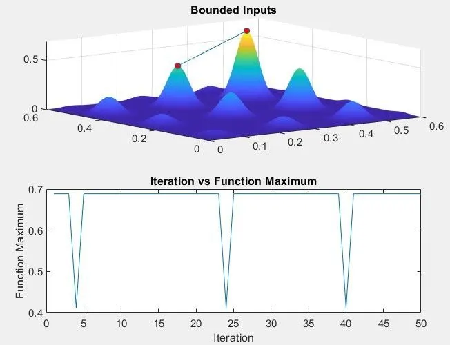
The optimum values were within limits failing to obtain the precise maxima
values.
Elapsed study time = 4.0090 (which is more than above study)
Study 3- Statistical Behavior of Increased Initial Population and
Bounded Values. In this study, the population size is increased
from 50 to 250
tic
options = optimoptions('ga');
options = optimoptions(options,'populationsize',250);
for i = 1:num_cases
[results,fopt(i)] = ga(@stalagmite,2,[],[],[],[],[0;0],[0.6;0.6],[],[],options);
xopt(i) = results(1);
yopt(i) = results(2);
end
study3_time = toc
figure(3)
subplot(2,1,1)
surf(x,y,-f)
shading interp
hold on
plot3(xopt,yopt,-fopt,'marker','o','markersize',5,'markerfacecolor','r')
title('Increased Initial Population')
subplot(2,1,2)
plot(-fopt)
title('Iteration vs Function Maximum')
xlabel('Iteration')
ylabel('Function Maximum')
In this case study, 'optimoptions' is used to increase the population
size to 250.
Storing the results in xopt,yopt & plotting the surface of x,y,-f
to get the 3D plot.
Study - 3 - Output>>>>>
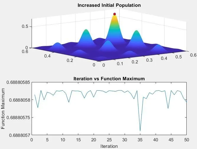
Elapsed Study Time = 23.1109
This case study took more to time for completion but was successful and
the correct maxima was found for the given stalagmite function.
Conclusion : Therefore, using this algorithm we conclude that by increasing the
population size we obtain a fairer accuracy in recognizing the optimum maxima value.
Q4. Any references?
Ans.
Genetic Algorithms - Introduction (tutorialspoint.com)