Project 2 - Rankine cycle Simulator
Rankine cycle
The Rankine cycle or Rankine Vapor Cycle is the process widely used by power plants such as coal-fired power plants or nuclear reactors. In this mechanism, a fuel is used to produce heat within a boiler, converting water into steam which then expands through a turbine producing useful work. This process was developed in 1859 by Scottish engineer William J.M. Rankine. This is a thermodynamic cycle which converts heat into mechanical energy—which usually gets transformed into electricity by electrical generation.
Rankine Cycle – Processes
In an ideal Rankine cycle, the system executing the cycle undergoes a series of four processes: two isentropic (reversible adiabatic) processes alternated with two isobaric processes:
- Isentropic compression
- Isobaric heat addition
- Isentropic expansion
- Isobaric heat rejection (in a heat exchanger)
Required Inputs:
Turbine Inlet temperature = 400° C
Turbine Inlet Pressure = 30 bars
Turbine Outlet Pressure = 0.05 bars = Condenser Inlet Pressure
MAIN PROGRAM
%RANKINE CYCLE SIMULATOR

clear all
close all
clc

%% The processes of the rankine cycle

%  1-2 : Isentropic Expansion in the turbine
%    2-3 : Isobaric Heat Rejection by the condenser
%      3-4 : Isentropic Compression in the pump
%        4-1 : Isobaric Heat Addition by the boiler

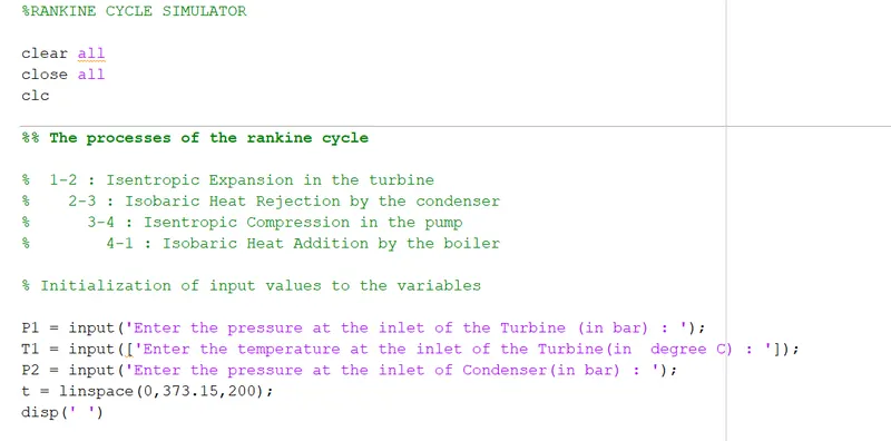
% Initialization of input values to the variables

P1 = input('Enter the pressure at the inlet of the Turbine (in bar) : ');
T1 = input(['Enter the temperature at the inlet of the Turbine(in  degree C) : ']);
P2 = input('Enter the pressure at the inlet of Condenser(in bar) : ');
t = linspace(0,373.15,200);
disp(' ')


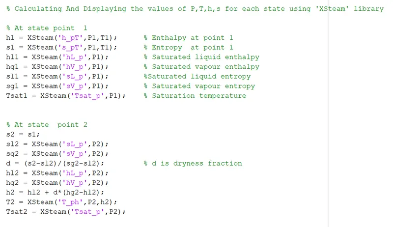
% Calculating And Displaying the values of P,T,h,s for each state using 'XSteam' library

% At state point  1
h1 = XSteam('h_pT',P1,T1);      % Enthalpy at point 1
s1 = XSteam('s_pT',P1,T1);      % Entropy  at point 1
hl1 = XSteam('hL_p',P1);        % Saturated liquid enthalpy
hg1 = XSteam('hV_p',P1);        % Saturated vapour enthalpy
sl1 = XSteam('sL_p',P1);        %Saturated liquid entropy
sg1 = XSteam('sV_p',P1);        % Saturated vapour entropy
Tsat1 = XSteam('Tsat_p',P1);    % Saturation temperature


% At state  point 2
s2 = s1;
sl2 = XSteam('sL_p',P2);
sg2 = XSteam('sV_p',P2);
d = (s2-sl2)/(sg2-sl2);         % d is dryness fraction
hl2 = XSteam('hL_p',P2);
hg2 = XSteam('hV_p',P2);
h2 = hl2 + d*(hg2-hl2);
T2 = XSteam('T_ph',P2,h2);
Tsat2 = XSteam('Tsat_p',P2);


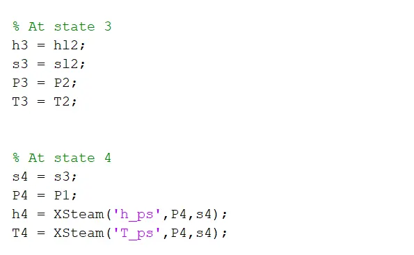
% At state 3
h3 = hl2;
s3 = sl2;
P3 = P2;
T3 = T2;


% At state 4
s4 = s3;
P4 = P1;
h4 = XSteam('h_ps',P4,s4);
T4 = XSteam('T_ps',P4,s4);

% Work and efficiency Calculations

% Work done by turbine
W_turbine = h1 - h2;

% Work done by pump
W_pump = h4 - h3;

% Net work dome
W_net = W_turbine - W_pump;

% Thermal efficiency
therm_eff = (1 - ((h2 - h3)/(h1 - h4)))*100;

% Back work ratio
back_wr = W_pump/W_turbine;

% Specific Steam Conductivity
ssc = 3600/W_turbine;


%% Plotting Of Different curevs


% Plotting T-s graph
figure(1), clf
hold on

% Saturation curve
for i = 1:length(t)
plot(XSteam('sL_T',t(i)),t(i),'g')
plot(XSteam('sV_T',t(i)),t(i),'g')
end

% Cycle
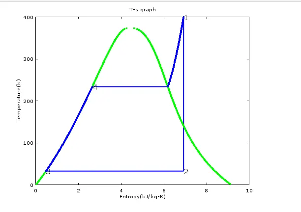
plot([s1 s2],[T1 T2],'linewidth',2)
text(s1,T1,'1','FontSize',15)
if d > 1
T3 = Tsat2;
plot([s2 sg2 s3 s4],[T2 Tsat2 T3 T4],'linewidth',2)
T2 = Tsat2;
text(s2,T2,'2','FontSize',15)
text(s3,T3,'3','FontSize',15)
else
plot([s2 s3 s4],[T2 T3 T4],'linewidth',2)
text(s2,T2,'2','FontSize',15)
text(s3,T3,'3','FontSize',15)
end
n = linspace(T1,T2,500);
for i = 1:length(n)
plot(XSteam('s_pT',P1,n(i)),n(i),'.','linewidth',2)
end

plot([sl1 sg1],[Tsat1 Tsat1],'linewidth',2)
text(sl1,Tsat1,'4','FontSize',15)
xlabel('Entropy(kJ/kg-K)')
ylabel('Temperature(k)')
title('T-s graph')


% h-s graph
figure(2), clf
hold on

% Saturation curve
for i = 1:length(t)
plot(XSteam('sL_T',t(i)),XSteam('hL_T',t(i)),'r.')
plot(XSteam('sV_T',t(i)),XSteam('hV_T',t(i)),'r.')
end

% Cycle
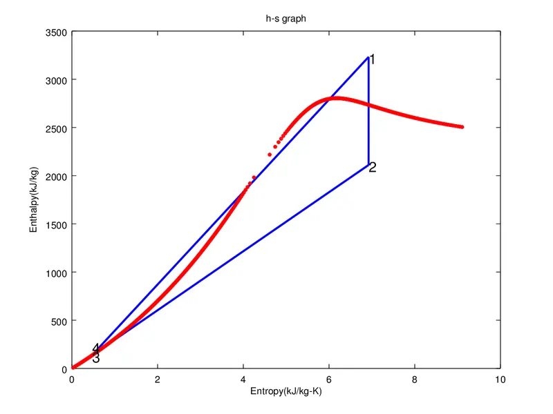
plot([s1 s2 s3 s4 s1],[h1 h2 h3 h4 h1],'linewidth',2)
text(s1,h1,'1','FontSize',15)

text(s2,h2,'2','FontSize',15)
text(s3,h3,'3','FontSize',15)
text(s4,h4+90,'4','FontSize',15)

xlabel('Entropy(kJ/kg-K)')
ylabel('Enthalpy(kJ/kg)')
title('h-s graph')

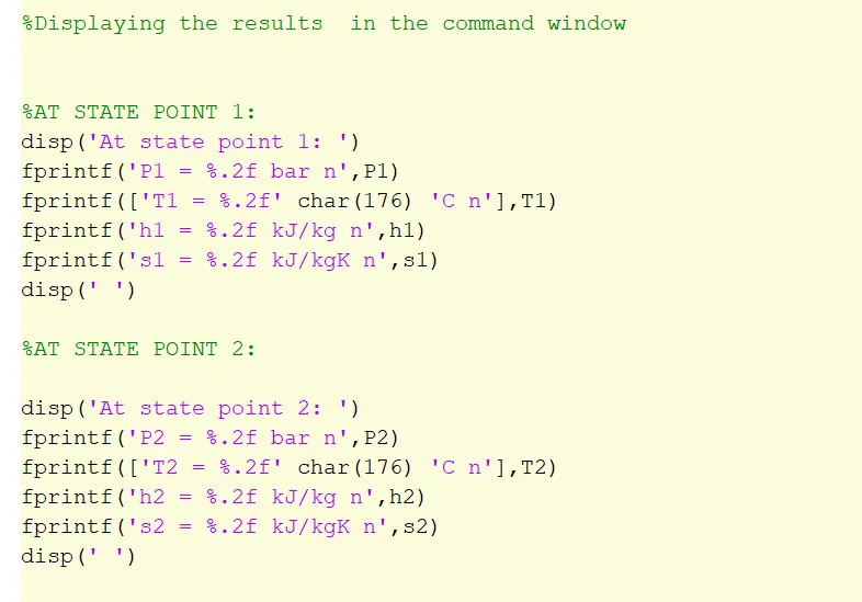
%Displaying the results  in the command window


%AT STATE POINT 1:
disp('At state point 1: ')
fprintf('P1 = %.2f bar n',P1)
fprintf(['T1 = %.2f' char(176) 'C n'],T1)
fprintf('h1 = %.2f kJ/kg n',h1)
fprintf('s1 = %.2f kJ/kgK n',s1)
disp(' ')

%AT STATE POINT 2:

disp('At state point 2: ')
fprintf('P2 = %.2f bar n',P2)
fprintf(['T2 = %.2f' char(176) 'C n'],T2)
fprintf('h2 = %.2f kJ/kg n',h2)
fprintf('s2 = %.2f kJ/kgK n',s2)
disp(' ')


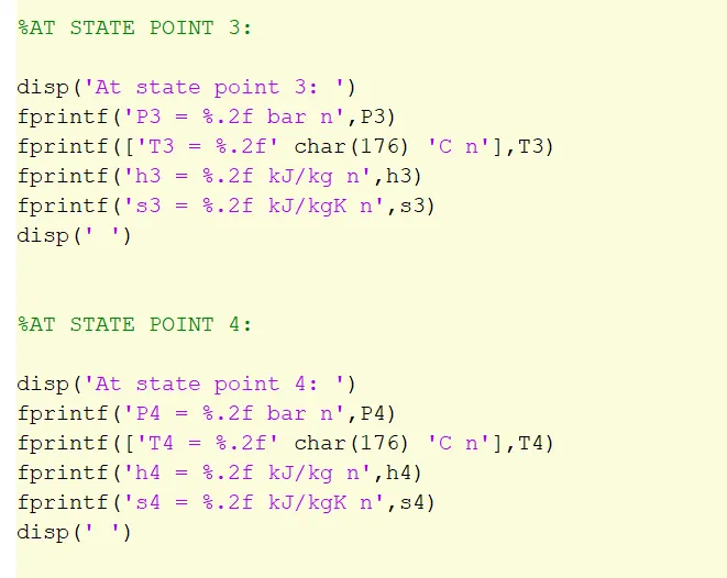
%AT STATE POINT 3:

disp('At state point 3: ')
fprintf('P3 = %.2f bar n',P3)
fprintf(['T3 = %.2f' char(176) 'C n'],T3)
fprintf('h3 = %.2f kJ/kg n',h3)
fprintf('s3 = %.2f kJ/kgK n',s3)
disp(' ')


%AT STATE POINT 4:

disp('At state point 4: ')
fprintf('P4 = %.2f bar n',P4)
fprintf(['T4 = %.2f' char(176) 'C n'],T4)
fprintf('h4 = %.2f kJ/kg n',h4)
fprintf('s4 = %.2f kJ/kgK n',s4)
disp(' ')


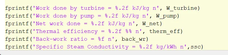
fprintf('Work done by turbine = %.2f kJ/kg n', W_turbine)
fprintf('Work done by pump = %.2f kJ/kg n', W_pump)
fprintf('Net work done = %.2f kJ/kg n', W_net)
fprintf('Thermal efficiency = %.2f %% n', therm_eff)
fprintf('Back-work ratio = %f n', back_wr)
fprintf('Specific Steam Conductivity = %.2f kg/kWh n',ssc)
DETAILED EXPLANATION OF THE CODE
STEP – 1
Starting the program with first manually passing the input values of ‘P1’, ‘T1’, ’P2’ in the command window. The values of ‘t’ are passed automatically with 200 values using ‘linspace’ command.
STEP – 2
Now, using the ‘XSteam’ library, the values of various physical parameters i.e. Enthalpy, Entropy, Saturated liquid/vapour – Enthalpy/Entropy and saturation temperature @ all 4 state points were calculated.
STEP – 3
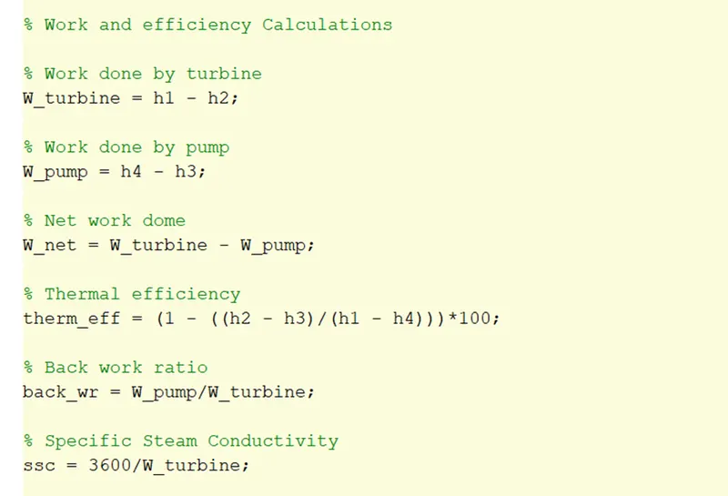
Now, using the basic calculations for work done for turbine and pump, the net work done, thermal efficiency and back work ratio is calculated.
STEP – 4
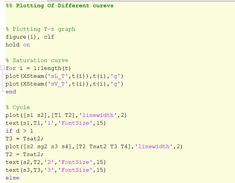
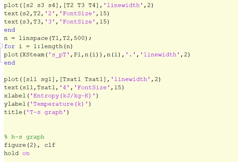
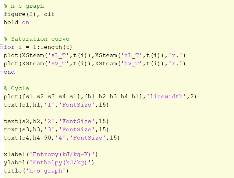
The ‘XSteam’ library function was used to plot the T-s curve at various temperatures. The curve was plotted along the state points.
STEP – 5
The various physical parameters for all 4 state points were displayed successfully in the command window.
STEP – 6
The final results ‘W_net’, ‘W_turbine , ‘W-pump’, ‘back-wr’ , ‘ssc’, ‘therm_eff’ were calculated and printed.
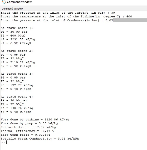
OUTPUTS :
Command Window Output
H-S Graph
T-S Graph
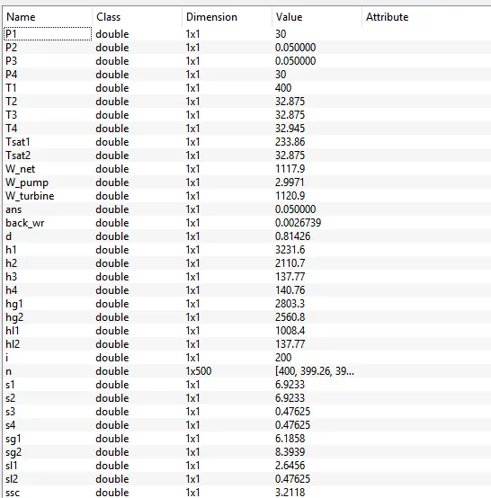
WORKSPACE OUTPUT