Week 4.1 - Genetic Algorithm

Pre-defined Function:

function [f] = stalagmite(input_vector)
x = input_vector(1);
y = input_vector(2);
x1 = (sin(5.1*pi*x+0.5))^6;
y1 = (sin(5.1*pi*y+0.5))^6;
x2 = exp(-4*log(2)*((x-0.0667)^2)/0.64);
y2 = exp(-4*log(2)*((y-0.0667)^2)/0.64);

f = -(x1*y1*x2*y2);
end

Code:

% Genetic Algorithm

% Defining search space( Creating 1D array)
x = linspace(0,0.5,100);
y = linspace(0,0.5,100);

% Number of cases
n = 70;

% Creating 2D array by meshing
[xx, yy] = meshgrid(x,y);

% Evaluating Stalagmite Function
for i= 1:length(xx)
    for j= 1:length(yy)
        input_vector(1)= xx(i,j);
        input_vector(2)= yy(i,j);

        f(i,j)= stalagmite(input_vector);
    end
end

% Study 1: statistical Behaviour

tic
for i= 1:n
    [inputs,fopt(i)]= ga(@stalagmite,2);
    % Storing the x and y values
    xopt(i) = inputs(1);
    yopt(i) = inputs(2);
end
study_time1 = toc;
figure(1)
subplot(2,1,1)
hold on
surfc(xx,yy,-f)
xlabel('x axis')
ylabel('y axis')
shading interp
plot3(xopt,yopt,-fopt,'Marker','O','MarkerSize',5,'MarkerFaceColor','r')
title('Unbounded Inputs')
subplot(2,1,2)
plot(fopt)
xlabel('Iterations')
ylabel('Function Maximum')

% Study 2 - Statistical Behaviour with Lower bound and Upper bound
tic
for i= 1:n
    [inputs,fopt(i)]= ga(@stalagmite,2,[],[],[],[],[0;0],[2;2]);
     % Storing the x and y values
    xopt(i) = inputs(1);
    yopt(i) = inputs(2);
end
study_time2 = toc;
figure(2)
subplot(2,1,1)
hold on
surfc(xx,yy,-f)
xlabel('x axis')
ylabel('y axis')
shading interp
plot3(xopt,yopt,-fopt,'Marker','O','MarkerSize',5,'MarkerFaceColor','b')
title('Bounded Inputs')
subplot(2,1,2)
plot(fopt)
xlabel('Iterations')
ylabel('Function Maximum')

% Study 3: Statistical Behaviour with Increasing Population

options = optimoptions('ga');
options = optimoptions(options,'PopulationSize',200);

tic
for i= 1:n
    [inputs,fopt(i)]= ga(@stalagmite,2,[],[],[],[],[0;0],[2;2],[],[],options);
     % Storing the x and y values
    xopt(i) = inputs(1);
    yopt(i) = inputs(2);
end
study_time3 = toc;
figure(3)
subplot(2,1,1)
hold on
surfc(xx,yy,-f)
xlabel('x axis')
ylabel('y axis')
shading interp
plot3(xopt,yopt,-fopt,'Marker','O','MarkerSize',5,'MarkerFaceColor','g')
title('Bounded Inputs with Increasing Population')
subplot(2,1,2)
plot(fopt)
xlabel('Iterations')
ylabel('Function Maximum')

Explanation:

• Define the search space i.e by creating 1D arrays by defining x and y using linspace
• Defining the no.of iterations as n= 70
• Creating 2D array by using meshgrid between x and y
• Evaluating the stalagmite function using a for loop and defining input vector
• Calling a pre defined function stalagmite
• assigning a function f that defines the stalagmite function as f(i,j)= stalagmite(input_vector)
• Study1 gives us the data about the statistical behaviour
• Using tic and toc cammands to know the execution time of the study1
• In the for loop an array is defined i.e inputs and fopt as a function of ga
• fopt gives the optimum value that the function predicts
• the syntax of the ga used here is simple i.e fun and nvars
• storing x and y values in xopt and yopt
• Creating 2 subplots, one gives the 3D plot and the other gives the 2D plot b/w no.of iterartions and function maximum
• In Study2, the syntax of the ga changes as we give the lower and upper bounds and leaving the linear inequalities as null vector.
• The same process for the plotting is repeated as done in the study1
• In Study3, the population size is increased so as to decrease the different maximas in different cases.
• The syntax of the ga changes, here the bounds are also added along with options. The nonlinear equalities and inequalities and the integer constrains are left as null vector.
• The same plotting is repeated for the study3 also.

Graphs:

Study1:

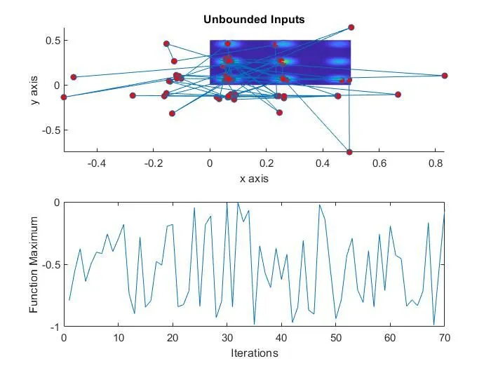
• Plotting the maximum values that the ga predicts
• The graph is all over the place, because of random sampling gives different results for each case.
• Takes the minimum time.

Study 2:

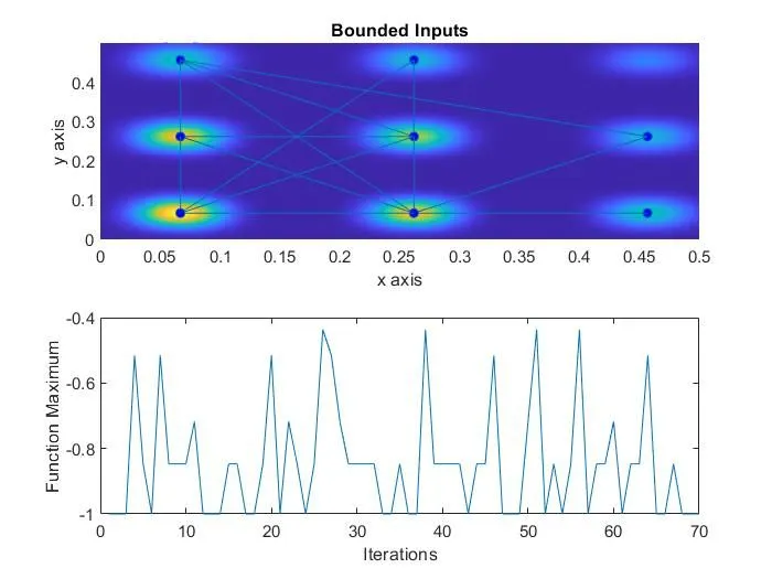
• It cares more time than study1
• The graph we get is more cleaner than study1.
• The function predicts that the maximum point is between a less no.of peaks, much better than previous code.
• It decreases the search space.

Study 3:

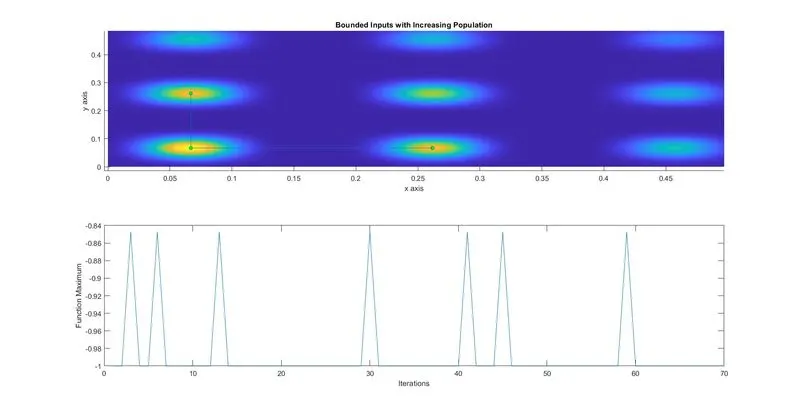
• This code takes the most time than the previous codes
• Maximum value is between much less than the previous peaks
• The minimum search space than the others.

Study_time1= 3.5458

Study_time2= 5.1565

Study_time3= 15.4267

Genetic Algorithm:

It works on the process of naturally selecting the fittest individual for reproduction and create the offsprings. It is used for solving both constarined and unconstrained optimization problems by selecting naturally. It starts by creating an intial population by selecting randomly. Then, the fitness of individuals is calculated. If the fitness satisfies the critereon then the function end else the selection of the individuals is done by genetic operator. It can be done by crossover operation or mutation operation. The crossover operator selects 2 individuals and swap a section of gene b/w them. Whereas, in mutation the selected individual undergoes mutation in genes. After these processes, these individuals again undergo fitness calculation and must satisfy the stop critereon. This process repeats untill the fitness matches the critereon.

1.x = ga(fun,nvars)
2.x = ga(fun,nvars,A,b)
3.x = ga(fun,nvars,A,b,Aeq,beq)
4.x = ga(fun,nvars,A,b,Aeq,beq,lb,ub)
5.x = ga(fun,nvars,A,b,Aeq,beq,lb,ub,nonlcon)
6.x = ga(fun,nvars,A,b,Aeq,beq,lb,ub,nonlcon,options)
7.x = ga(fun,nvars,A,b,Aeq,beq,lb,ub,nonlcon,intcon)
8.x = ga(fun,nvars,A,b,Aeq,beq,lb,ub,nonlcon,intcon,options)

The syntaxes used here in study1, study2 and study3 are 1,4 and 8 respectively.