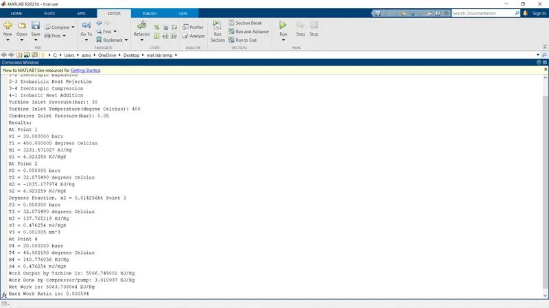
Project 2 - Rankine cycle Simulator

Code:

% Rankine Cycle Simulator

close all
clear all
clc

% Description
fprintf('Rankine Cycle Simulator \n\n')
fprintf('1-2 Isentropic Expansion \n')
fprintf('2-3 Isobaricic Heat Rejection \n')
fprintf('3-4 Isentropic Compression \n')
fprintf('4-1 Isobaric Heat Addition \n')

% Getting Inputs

P1 = input('Turbine Inlet Pressure(bar): ');
T1 = input('Turbine Inlet Temperature(degree Celcius): ');
P2 = input('Conderser Inlet Pressure(bar): ');
% Results
fprintf('Results: \n')

% Gathering Saturation Temperatures at P1 and P2
Sat_T_P1 = XSteam('Tsat_p',P1);
Sat_T_P2 = XSteam('Tsat_p',P2);

% Gathering Enthaply and Entropy at Saturation Points( on the vapour dome/curve)
% Point 1
Hg_1 = XSteam('hV_p',P1);
Sg_1 = XSteam('sV_p',P1);
% Point 2
Hg_2 = XSteam('hV_p',P2);
Sg_2 = XSteam('sV_p',P2);
% Point 3
Hf_3 = XSteam('hL_p',P2);
Sf_3 = XSteam('sL_p',P2);
% Point 4
Hf_4 = XSteam('hL_p',P1);
Sf_4 = XSteam('sL_p',P1);

% Calculating Enthalpy and Entropy at Point 1
H1 = XSteam('h_pT',P1,T1);
S1 = XSteam('s_pT',P1,T1);

% Calculating Temperature, Enthalpy and Entropy at Point 2
% entropy
S2 = S1; % isentropic process
% dryness fraction
if (S2<Sg_2)
    x2 = (S2-Sf_3)/(Sg_2-Sf_3); %(since, sf2=sf3)
else
    x2 = 1;
end
% temperature
CP2_V = XSteam('CpV_p',P2);
if(x2<1)
    T2 = Sat_T_P2;  
else
    T2 = (Sat_T_P2+273)*exp((S2-Sg_2)/CP2_V);
T2 = T2-273;

end
% Enthalpy
if(x2<1)
H2 = Hf_3 + x2*(Hf_3-Hg_2);
else
    H2 = XSteam('h_pT',P2,T2);
end

% Calculating Properties at Point 3
% Pressure
P3 = P2; % isobaric process
% Volume
V3 = XSteam('vL_p',P3);
% Temperature
T3 = Sat_T_P2;
% Enthalpy
H3 = Hf_3;
% Entropy
S3 = Sf_3;

% Calculating Properties at Point 4
% Pressure
P4 = P1;
% Entropy
S4 = S3;
% Volume
V3 = XSteam('vL_p',P3);
% Work done by compressor/pump
Wp = V3*(P4-P3)*100; % since, pressure is in bar, we multiply Wp with 100
% Enthalpy 
H4 = Wp + H3;
% Temperature
CP1_L = XSteam('CpL_p',P1); 
T4 = (Sat_T_P1+273)/exp((Sf_4-S4)/CP1_L);
T4 = T4-273;

% Displaying Properties 
fprintf('At Point 1 \n')
fprintf('P1 = %f bars \n',P1)
fprintf('T1 = %f degrees Celcius \n',T1)
fprintf('H1 = %f KJ/Kg \n',H1)
fprintf('S1 = %f KJ/KgK \n',S1)
fprintf('At Point 2 \n')
fprintf('P2 = %f bars \n',P2)
fprintf('T2 = %f degrees Celcius \n',T2)
fprintf('H2 = %f KJ/Kg \n',H2)
fprintf('S2 = %f KJ/KgK \n',S2)
fprintf('Dryness Fraction, x2 = %f',x2)
fprintf('At Point 3 \n')
fprintf('P3 = %f bars \n',P3)
fprintf('T3 = %f degrees Celcius \n',T3)
fprintf('H3 = %f KJ/Kg \n',H3)
fprintf('S3 = %f KJ/KgK \n',S3)
fprintf('V3 = %f mm^3 \n',V3)
fprintf('At Point 4 \n')
fprintf('P4 = %f bars \n',P4)
fprintf('T4 = %f degrees Celcius \n',T4)
fprintf('H4 = %f KJ/Kg \n',H4)
fprintf('S4 = %f KJ/KgK \n',S4)

% Plotting
% Calculating for Saturated Liquid and Vapour Lines
T = linspace(1,T1,1000);
for i = 1:length(T)
    H_L(i) = XSteam('hL_T',T(i));
    H_V(i) = XSteam('hV_T',T(i));
    S_L(i) = XSteam('sL_T',T(i));
    S_V(i) = XSteam('sV_T',T(i));
end


% T-S Diagram
figure(1)
hold on
plot([S1 S2],[T1 T2],'color','r','LineWidth',2)
text(S1,T1,'1')
text(S2,T2,'2')
text(Sg_2,Sat_T_P2,'2*')
plot([S2 S3],[T2 T3],'color','r','LineWidth',2)
text(S3,T3,'3')
plot([S3 S4],[T3 T4],'color','r','LineWidth',2)
text(S4,T4,'4')
plot([S4 Sf_4],[T4 Sat_T_P1],'color','r','LineWidth',2)
text(Sf_4,Sat_T_P1,'4*')
plot([Sf_4 Sg_1],[Sat_T_P1 Sat_T_P1],'color','r','LineWidth',2)
text(Sg_1,Sat_T_P1,'1*')
plot([Sg_1 S1],[Sat_T_P1 T1],'color','r','LineWidth',2)
plot(S_L,T,'LineStyle','--','Color','b')
plot(S_V,T,'LineStyle','--','Color','b')
title('T-S Diagram')
xlabel('Specific Entropy(KJ/KgK)')
ylabel('Temperature(degrees Celcius)')


% H-S Diagram
figure(2)
hold on
plot([S1 S2],[H1 H2],'color','r','LineWidth',2)
text(S1,H1,'1')
text(S2,H2,'2')
text(Sg_2,Hg_2,'2*')
plot([S2 S3],[H2 H3],'color','r','LineWidth',2)
text(S3,H3,'3')
plot([S3 S4],[H3 H4],'color','r','LineWidth',2)
text(S4,H4,'4')
plot([S4 Sf_4],[H4 Hf_4],'color','r','LineWidth',2)
text(Sf_4,Hf_4,'4*')
plot([Sf_4 Sg_1],[Hf_4 Hg_1],'color','r','LineWidth',2)
text(Sg_1,Hg_1,'1*')
plot([Sg_1 S1],[Hg_1 H1],'color','r','LineWidth',2)
plot(S_L,H_L,'LineStyle','--','Color','b')
plot(S_V,H_V,'LineStyle','--','Color','b')
title('H-S Diagram')
xlabel('Specific Entropy(KJ/KgK)')
ylabel('Specific Enthalpy(KJ/Kg)')


% Work Done, Heat and Back Work Ratio  

Wt = H1-H2;
fprintf('Work Output by Turbine is: %f KJ/Kg \n',Wt)
fprintf('Work Done by Compressor/pump: %f KJ/Kg \n',Wp)
Wnet = Wt-Wp;
fprintf('Net Work is: %f KJ/Kg \n',Wnet)
Back_Work_Ratio = Wp/Wt;
fprintf('Back Work Ratio is: %f \n',Back_Work_Ratio)

Explanation:

• Study the XSteam function and know all the syntaxes, functions and inputs for the function.
• Closing all figures, clearing workspace and clearing command window
• Displaying all the description about the processes in the cycle
• Getting the inputs by using the input command. These inputs are entered in the command window
• Gathering the Saturation temperatures at Pressures P1 and P2 and storing them in variables Sat_T_P1 and Sat_T_P2.
• The saturation temperatures are obtained by using the XSteam function.
• Gathering the Enthalpy and Entropy at Saturation points by using the XSteam function and storing in their respective variables
• Gathering and calculating all the required properties at all the four stages of the rankine cycle.
• The required properties are enthalpy and entropy at all 4 points
• Displaying all the properties calculated and gathered in the command window using the fprintf command
• All the calculations are done by using the thermodynamic equations
• The temperature trace is taken by using linspace command. The Temperature is divided into 1000 between 1 and T1
• A forloop is created to get the saturated liquid and vapour points by using XSteam function at T(i) temperature.
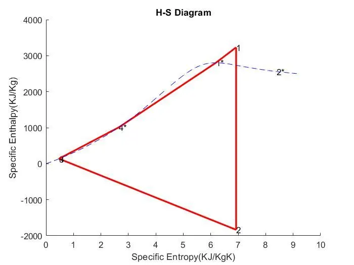
• For plotting the Vapour dome/curve, we use liquid and vapour saturation points of enthalpy and entropy
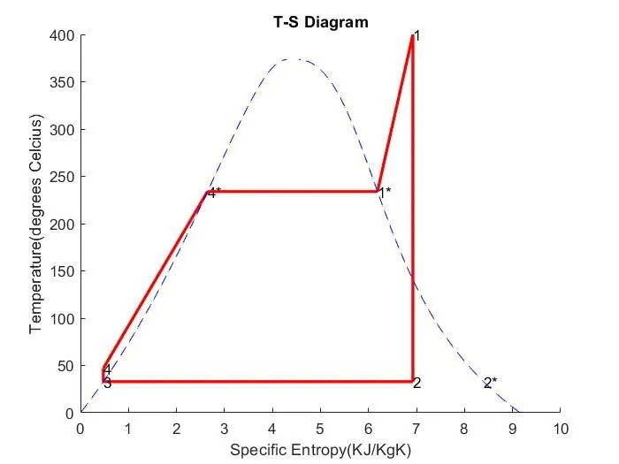
• Plotting the T-S diagram and H-S diagram by using plot command by taking entropy on x axis and temperature and enthalpy on y axis respectively
• Use text command to name the points 1,2,2*,3,4,4* and 1*.
• Calculate the net work output and back work ratio.
• Use the fprintf command to display the turbine work, pump work, net work and back work ratio

Graphs:

T-S Diagram:

H-S Diagram:

Output Screen: