Week 3 - Solving second order ODEs

Code:

% Simple Pendulum( It is an example for a second order ODE)

% Inputs(damping coeff,b; acceleration due to gravity,g; length from fixed point to center of mass,l; mass,m)

b = 0.05;
g = 9.81;
l = 1;
m = 1;

% Initial conditions( for dispalcement and velocity)
theta_T= [0;3];

% Time Points 
t_span = linspace(0,20,200);

% Solving ODE
% calling a pre-defined function i.e simple_pendulum 
[t,results]= ode45(@(t,theta) simple_pendulum(t,theta,b,g,l,m),t_span,theta_T);

% Plotting
figure(1)
%  For displacement we take results(:,1)
plot(t,results(:,1),'Color','r')
hold on
% For velocity we take results(:,2)
plot(t,results(:,2),'Color','b')
xlabel('time')

% Animation for SImple Pendulum
% Fixed Point
x0=0;
y0=0;

ct=1;

for i= 1:length(t)
    x1 = l*sin(results(i,1));
    y1 = -l*cos(results(i,1));

    figure(2)
    

    % plane of fixed point
    plot([-1 1],[0 0],'LineWidth',5,'color',[0 0 0])
    axis([-2 2 -2 1])
    % Line representing the string og pendulum
    line([x0 x1],[y0 y1],'linewidth',2,'color','b')
    hold on
    % Fixed point of the string
    plot(x0,y0,'O','MarkerSize',1,'MarkerFaceColor','g')
    % mass at other end of string
    plot(x1,y1,'O','MarkerSize',10,'MarkerFaceColor','r')
    hold off
    grid on
     M(ct)= getframe(gcf);
     ct= ct+1;
end

movie(M)
videofile = VideoWriter('simple_pendulum_animation.avi','Uncompressed AVI');
open(videofile)
writeVideo(videofile,M)
close(videofile)

Function :

function [dtheta_dt]= simple_pendulum(t,theta,b,g,l,m)

theta1 = theta(1);
theta2 = theta(2);
dtheta1_dt = theta2;
dtheta2_dt = -(b/m)*theta2-(g/l)*sin(theta1);

dtheta_dt = [dtheta1_dt; dtheta2_dt];
end

Google drive link : https://drive.google.com/file/d/1X7wfyAbbj_qnbjHIEMpbUsTYTpMKw1J5/view?usp=sharing

Graph :

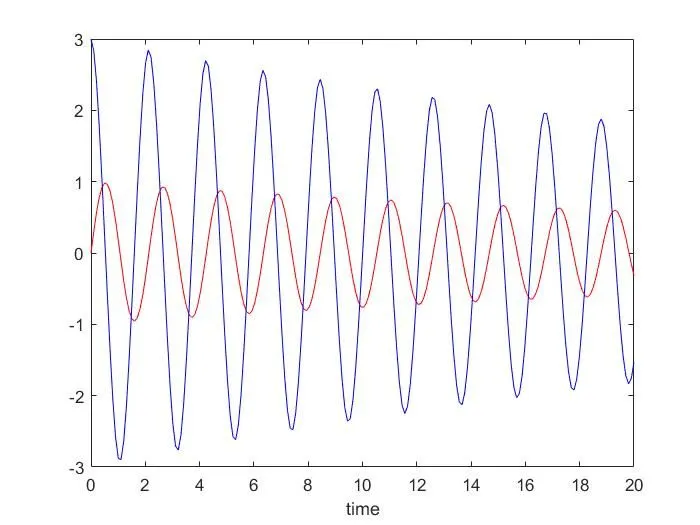
Explanation :

The given second order ODE is converted into an equation, by substituting theta with theta1 and derivative of theta1 with theta2. To get a solution vector easily by substituting. The inputs, initial conditions and time span are defined as given in the problem. A function is predefined that acts as an input in the ode45 function. The predefined function is obtained from the equation from before. The ode45 function is written with it's main inputs as t and theta. The time of intergration and initial conditions are also given in the ode45 function. Plotting of the graph is done by using the plot command by taking time on x axis and angular displacement and angular velocity which is the results of the ode function. The first coloumn of the results is displacement and the second coloumn of the results is velocity. The animation of the simple pendulum is obtained by using for loop. First, the fixed point is defined as x0 and y0. Later, the other end of the pendulum is defined by x1=l*sin(results(i,1)) and y1=l*cos(results(i,1)). The plane of fixed point is defined and the limits of axis are alos defined. line command is used to plot the string of pendulum. The mass is obtained by creating a sphere as a marker. A counter is also provided to get each and every frame. Before ending the for loop, we define ct= ct+1 so as to get every frame in the next loop. M is defined as a funtion of ct which is later used to get the animated videofile. Movie command is used to view a movie of the frames. A videofile is created by using videowriter command which defines it's name and the type of file. Open and close command are used to open the video and close it after viewing.

Errors: The errors faced while executing the program are getting only a single graph when hold on command is not used and for not using hold off command during the animation.