Week 4.1 - Genetic Algorithm

Aim : To optimise the stalagmite function and find the global maxima of the function.

Explanation of genetic algorithm and syntax for it:

What is Genetic algorithm?

• It is a search based optimisation technique which works on the principle of genetics and Natural selection proposed by Charles Darwin.It is a method for solving both constrained and unconstrained optimisation problems.
• It always minimize the function.

How it works?

• The algorithm repeatedly modifies a population of individual solutions. At each step, the genetic algorithm randomly selects individuals from the current population and uses them as parents to produce the children for the next generation. Over successive generations, the population "evolves" toward an optimal solution.

It is done in few steps as given below

1. Initialisation

In this step ,first population size is decided. Higher the population size more is the combination and we will get more accurate result.

2. Selection

In this step parents are selected from the sample data points and the main objective of this step is to select the highle fit individuals.

3. Cross over

In this step parents are taken and children are produced from them by interchanging their genes.

4.Mutation

To maintain the diversity, mutation is carried out from one generation of population of chromosomes to next generation.

If mutation is not performed, the chromosomes will become similar to each other,convergence will take place soon which results in local minima.

For which problems GA can be applied?

• It can be applied to solve problems which are not well suited for standard optimization algorithms, including the problems in which the objective function is discontinuous, non-differentiable or highly non-linear.

What is the difference between classical algorithm and genetic algorithm

• Classical Algorithm	Genetic Algorithm
  It Generates a single point at each iteration and sequence of points approaches an optimal solution.	Generates a population of points at each iteration and the best point in the population approaches an optimal solution.

SOME OF THE MAIN SYNTAX OF GA GIVEN ARE BELOW

x = ga(fun,nvars)
x = ga(fun,nvars,A,b)
x = ga(fun,nvars,A,b,Aeq,beq)
x = ga(fun,nvars,A,b,Aeq,beq,lb,ub)
 

%stalagmite function

function   [f] = stalagmite(input_vector)   %function 'stalagmite' which takes 'input_vector' as input
x=input_vector(1);                          % first value of input_vector is stored in x
y=input_vector(2);                          % second value of input_vector is stored in y
f1x=(sin(5.1*pi*x+0.5))^6;                % term1 i.e f1x=(sin(5.1*pi*x+0.5))^6
f1y=(sin(5.1*pi*y+0.5))^6;                % term2 i.e f1y=(sin(5.1*pi*y+0.5))^6
f2x=exp(-4*log(2)*((x-0.0667)^2/0.64));   % term3 i.e f2x=exp(-4*log(2)*((x-0.0667)^2/0.64))
f2y=exp(-4*log(2)*((y-0.0667)^2/0.64));   % term4 i.e f2y=exp(-4*log(2)*((y-0.0667)^2/0.64))
f=-f1x*f1y*f2x*f2y;                       % calculation of f=term1*term2*term3*term4
end                                       % termination of function

%optimisation coding
clear all               % removes all variables from the workspace.
close all               % Close figures
clc                     % clear screen

%defining our search space
x=linspace(0,0.6,150);  % returns a row vector of 150 evenly spaced points between 0 and  0.6    
y=linspace(0,0.6,150);  % returns a row vector of 150 evenly spaced points between 0 and 0.6 


%creating the two dimensional mesh
[xx,yy]=meshgrid(x,y);  % returns 2-D grid coordinates based on the coordinates contained in vectors x and y

%% evaluating the stalagmite function
 

% generating the plot of stalagmite function using nested loop
% using the nested loop for xx and yy 
for i=1:length(xx)       
    for j=1:length(yy)

%creating a row vector which have 2 columns        
input_vector(1)=xx(i,j);
input_vector(2)=yy(i,j);

% calculating the value of 'f' from the given stalagmite function 
f(i,j) = stalagmite(input_vector);
    end   % termination of j loop
end       % termination of i loop


surfc(xx,yy,-f)                 % creates a three-dimensional surface plot 
xlabel('x value')              % labelling x axis as 'x value'
ylabel('y label')              % labelling y axis as 'y value'
shading interp                 % shades the curves in a plot
[input,fval]=ga(@stalagmite,2); % performing genetic algorithm

Explanation of stalagmite function

• program starts with clear all, close all and clc which clears the workspace ,closes all the previous curves and clears the screen respectively.
• one dimensional array is created for x and y by using the linspace command.
• By using the meshgrid command 2 dimensional array is created.
• To evaluate the stalagmite function we are creating the nested loop .
• Then for each value of x and y an array is created that is input_vector.
• The stalagmite function is given which takes the input_vector as input and calculate the value of f.
• A separate stalagmite function is created where f1x,f1y,f2x and f2y terms are calculated by using the input_vector and finally the value of f is find by using the relation f=f1x*f1y*f2x*f2y
• A 3D plot is created by using the surfc command but in the graph unwanted lines are shown so to remove them we use 'shading interp ' command and then at last the genetic algorithm is used which takes the function handle stalagmite as input along with number of variables and find the value of x and y where the stalagmite function is minimum by default because it only finds the minimum value of the function and also the minimum value of 'f' is calculated which is stored in 'fval'.
• so a -ve sign is put before 'f' in the stalagmite function to find the maxima instead of minima.

OUTPUT OF THE PROGRAM

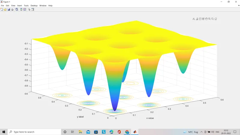
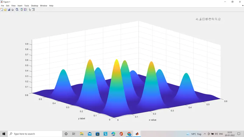
• This 3d graph is showing the local minimas and global minima it is when we do not put negative sign in the stalagmite function so to convert it into the 3d graph of local maxima and global maxima we will put negative sign in 'f' in the stalagmite function as well as in th surf command and then we get the graph as shown below

Observation

Every time we run the GA code it is giving the different results. So this brings the interesting question in our mind then how GA is useful if it is giving me different results every time .

So to understand this we are doing 3 studies which I have given below

 %optimisation coding
clear all               % removes all variables from the workspace.
close all               % Close figures
clc                     % clear screen

%defining our search space
x=linspace(0,0.6,150);  % returns a row vector of 150 evenly spaced points between 0 and  0.6    
y=linspace(0,0.6,150);  % returns a row vector of 150 evenly spaced points between 0 and 0.6 


%creating the two dimensional mesh
[xx,yy]=meshgrid(x,y);  % returns 2-D grid coordinates based on the coordinates contained in vectors x and y

%% evaluating the stalagmite function
 

% generating the plot of stalagmite function using nested loop
% using the nested loop for xx and yy 
for i=1:length(xx)       
    for j=1:length(yy)

%creating a row vector which have 2 columns        
input_vector(1)=xx(i,j);
input_vector(2)=yy(i,j);

% calculating the value of 'f' from the given stalagmite function 
f(i,j) = stalagmite(input_vector);
    end   % termination of j loop
end       % termination of i loop

%% study1
num_cases=50                % counter for iterations      
tic                         % Start stopwatch time
for i=1:num_cases           % iterations 
    [input,fopt(i)]=ga(@stalagmite,2)  %genetatic algorithm function to find the minimum value (by default)
    xopt(i)=input(1);                  % stores the 1st optimum x value 
    yopt(i)=input(2);                  % stores the 2nd optimum y value
end                                    % termination of loop
study_time=toc                         % Read elapsed time from stopwatch
figure(1)                              % create a figure window
subplot(2,1,1)                         % divides the current figure into an 2 by 1 grid
hold on                                % hold the previous plots
surf(x,y,-f)                           % create a 3d plot 
shading interp                         % shade the contours
plot3(xopt,yopt,-fopt,'marker','o','MarkerSize',5,'MarkerFaceColor','r')  % create the plot 
title('unbounded inputs')              % add title 
subplot(2,1,2)                         % creates the subplot
plot(-fopt)                            % plot the optimized function
xlabel ('iteration')                   % labelling x as iteration
ylabel(' function maxima')             % labelling y as function maxima

%% study 2

num_cases=50                               
tic  
% calling the ga function with bounded condition
% algorithm
for i=1:num_cases                      
    [input,fopt(i)]=ga(@stalagmite,2,[],[],[],[],[0;0],[1;1])
    xopt(i)=input(1);                     
    yopt(i)=input(2);
end
study_time=toc

% plotting the graph for study 2
figure(2)
subplot(2,1,1)
hold on
surf(x,y,-f)
shading interp
plot3(xopt,yopt,-fopt,'marker','o','MarkerSize',5,'MarkerFaceColor','r')
title('Bounded inputs')
subplot(2,1,2)
plot(-fopt)
xlabel ('iteration')
ylabel(' function max')



%% Study 3
% increasing the ga iterations
options=optimoptions('ga');
options=optimoptions(options,'populationSize',500)
 
% calling ga with bounded condition and increased iteration
tic
for i=1:num_cases
    [input,fopt(i)]=ga(@stalagmite,2,[],[],[],[],[0;0],[1;1],[],[],options)
    xopt(i)=input(1);
    yopt(i)=input(2);
end
study_time=toc

% plotting the study 3
figure(3)
subplot(2,1,1)
hold on
surf(x,y,-f)
shading interp
plot3(xopt,yopt,-fopt,'marker','o','MarkerSize',5,'MarkerFaceColor','r')
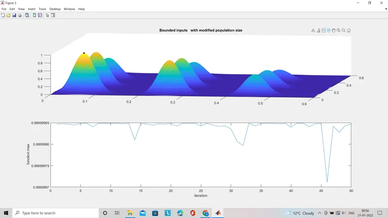
title('Bounded inputs   with modified population size')
subplot(2,1,2)
plot(-fopt)
xlabel ('iteration')
ylabel(' function max')

EXPLANATION OF CODE

• As we have noticed that every time we run the ga code we get different results so one question arise in mind how ga is useful if it is showing the different results
• To demonstrate it we first look at the statistical behaviour of ga code.
• We first start the code with as usual commands i.e clear all ,close all, clc.
• Then x and y are created (Remember: It does not define the workspace for genetic algorithm(ga) because ga does not know that this is actually the workspace which means it does not know that the value of x and y can go beyond 0.6 and 0.
• x and y are only the input arrays created.
• Then num_case gives the idea that ga willl run 50 times here.
• Then we have the stalagmite function which basically generates the stalagmite function.

• STUDY 1
• This is to just calling ga and passing the no of variables as input and storing x values and y values and also the optimum value which function predicts
• After that we open a new figure window and then create the subplot inside it.
• First plot is surface of stalagmite function.
• Plots3 command is used to plot x and y and optimum function value that ga predicts over 50 studies this helps us to visualize how the algorithm is working.
• To make it more clear 2nd subplot is created for optimum value as the function of iteration.
• To measure the time taken by study we are using tic and toc command.
• then the study 1 is evaluated and result is shown below

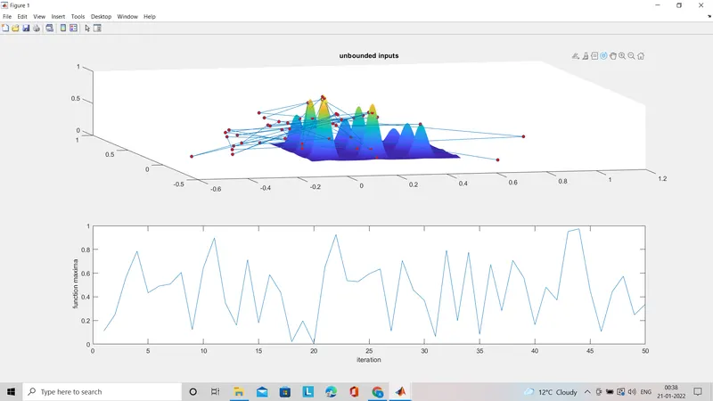
OBERVATION : Here in the graph we have noticed that maximum values of ga are plotted and its all over the place and this happens due to the random sampling as we get different values when we run the code different times and to visualize it clearly we can see the second subplot which shows that maximum value of function lie between o and 1 and this result is not correct.

Solution: Set up the bounds for the variables as the values of x and y were going beyond 0 and 0.6.

STUDY 2

• Here the only changes made is in the function definition of ga.
• Tic and toc command will show the timing and results are also obtained and this time plot looks little bit clear.

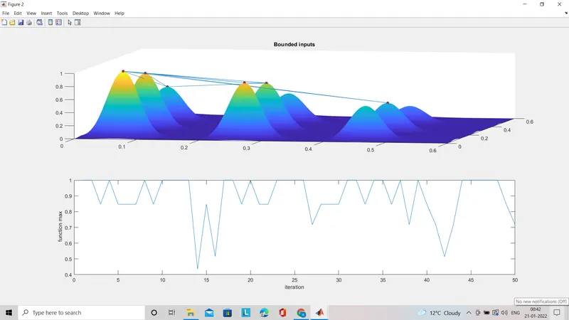
Observation: This time it is observed that the maximum point is between 5 peaks that we see in 3d graph.

and the maximum value is between 0.45 and 1 (narrow range)

Now th only thing we have to do is to reduce the search space which depends on what type of problem we are working.

STUDY 3

• In addition to specify the bonds we are going to change the initial population size .
• By default ga takes 50 as the no of samples .
• Since there are two variables so there are 50 sets of two random variables .
• If our population is too small it will not find the global maxima but it wil find the local maxima
• So we are increasing the size of population tpo 170 which slows down the ga which is seen by tic toc command.
• So as the number of iteration increases the more accurate the value will come.
• here this study takes 18.55 seconds which is more than the previous studies.

REFERENCE

https://in.mathworks.com/help/gads/ga.html#mw_f8e8d81b-aba1-4254-9f1a-cf93ff0ccc2b

https://skill-lync.com/student-projects/GENETIC-ALGORITHM-USING-MATLAB-38665

https://in.mathworks.com/help/gads/ga.html

ERRORS:

I got stuck how to find the maximum instead of minima as my graph was showing the downward curves which i have overcome by putting a negative sign before the ' f ' ,otherwise i did not find the error this time