Week 3 - Solving second order ODEs

% ODE function defination
function [dtheta_dt] =ode_fun(t,theta,b,g,l,m) % function ode_fun with input parameters

% converting the 2nd ODE into two 1st ODE
% theta is taken as solution vector
%clubbing theta1 and theta2 into variable called theta
theta1=theta(1); % 1st value of theta
theta2=theta(2); % 2nd value of theta
dtheta1_dt=theta2; % 1st ODE
dtheta2_dt=-(b/m)*theta2 - (g/l)*sin(theta1); % 2nd ODE
dtheta_dt=[dtheta1_dt;dtheta2_dt]; %combining theta1 &theta2 into an array
end %closing the function

%% explanation
* ode_fun is the function defination having input parameters
* t,theta,b,g,land m are the input parameters
* In this separate function we have converted the given second order
differential equation into two 1st order differential equations
* theta is taken as solution array which contain 2 values theta1 and theta2
* dtheta1_dt and dtheta2_dt are the two 1st order ODEs
* at last both the 1st order ODEs are clubbed into one array i.e dtheta_dt

clear all % clear the workspace
close all % clear all the previous graphs
clc % clear the screen

% input parameters
b=0.05; % damping coefficient
g=9.8; % acceleration due to gravity
l=1; % length of the pendulum
m=1; % mass of the bob

t_span=linspace(0,20,400) % time span
theta_0 = [0;3] % initial values of displacement and velocity

%solving the differential equation using ode45
[t,results]= ode45(@(t,theta) ode_fun(t,theta,b,g,l,m), t_span, theta_0)
%%syntax of ode45
%[tsol,ysol]= ode45(@(t,y) odefun(t,y), t_span, y0)
% where
% [tsol ,ysol]: solution vectors
% ode45 : inbuilt solver for first order differential equation
% @(t,y) : independent and dependent variable respectively
% odefun(t,y) : function that returns dy=F(t,y)
% t_span : time span or time integration
% y0 : initial condition

%plotting
figure(1) % creating the figure for displacement,velocity vs time graph
plot(t,results) % plotting the graph between t and results (i.e displacement and velocity)
xlabel('time'); % naming x axis
ylabel('displacement and velocity'); % naming y axis
grid on % switch on the grids in graph

%% creating the annimation for pendulum
ct=1; % counter to count the frames
theta_disp=results(:,1) % variable that stores a displacement value
for i=1:length(theta_disp) % loop
theta_new=theta_disp(i) % variable that stores the value of displacement
x0=0; % initial x coordinate for straight line
y0=0; % initial y coordinate for straight line
y1=-l*cos(theta_new); % final y coordinate for straight line
x1=l*sin(theta_new); % final x coordinate for straight line

figure(2)
plot([-1 1],[0 0],'Color','g','linewidth',5) %plotting the straight fixed line
hold on % hold or retain the current plot
plot([x0 x1],[y0 y1],'linewidth',3,'color','r') % plot straight line of pendulum
hold on % hold or retain the current plot
plot(x1, y1,'o','markers', 15,'markerfacecolor','r','markeredgecolor','b') % plot the bob
hold off % do not retain the previous plots of bob
grid on % switch on the grids
axis([-1.5 1.5 -2 0.5]) % set the x and y axis limits
M(ct)=getframe(gcf) % captures the figures as movie frames
ct=ct+1 % increment of the counter by 1

end % closing the loop

% creating the video annimation
movie(M); % creates the movie of frames captured
videofile = VideoWriter('pendulum annimation.avi','Uncompressed AVI') % creates a VideoWriter object to write video data to an AVI file
open(videofile); % Open file in appropriate application
writeVideo(videofile,M) % writes data from an array to the video file
close(videofile) % Close file after writing video data

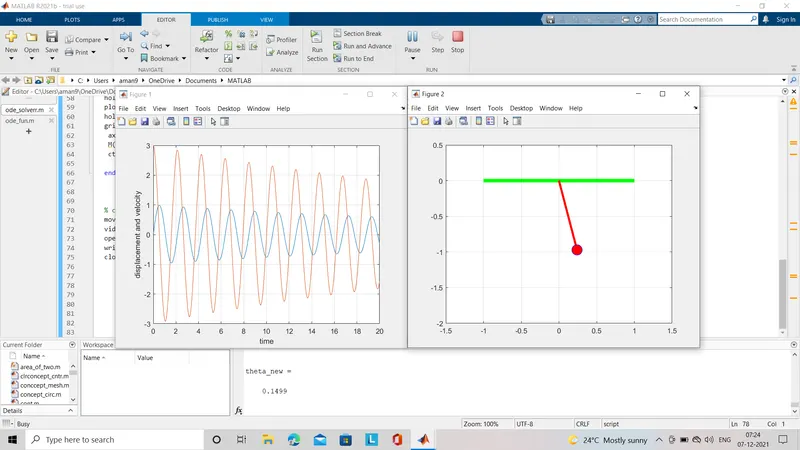
%graphs of output is attached below

%% errors faced during the execution of program
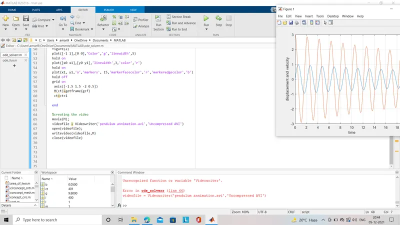
1. unrecognized function Videowriter is used instead of VideoWriter
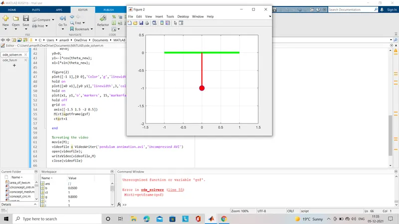
2. Unrecognized variable gsf is used instead of gcf in getframe

% how errors has overcome
1. Videowriter spelling is replaced by VideoWriter
2. gsf is replaced by gcf in getrame

screenshots of errors are attached

%% explanation of program
% in this program we have learnt how to solve the second order differential equation using ode45
here the 2nd order differential equation for simple pendulum was given and we are solving it for theta and rate at which the theta value is changing i.e velocity
%here b,g,l and m are used as input parameters and ode system is the
function of t and theta
% we are using a inbuilt function i.e ode45 to solve the differential equation here
%for that first we have to convert the 2nd order ODE into two 1st order
%ODEs which is done in separate function named ode_fun
%then once the two 1st order equations are formed then they are written in
%matrix form
%where theta will be taken as the solution vector which contains theta1 and
%theta2

% graph between the displacement,velocity and time is made and then the
annimation of pendulum is made
%where movie command used to captures the frames and create a movie
%VideoWriter- creates a VideoWriter object to write video data to an AVI file
%videofile is opened in appropriate application by using 'open' command
% VideoWriter writes data from an array to the video file and videofile is closed by using the close command

link for ANNIMATION OF PENDULUM is given below
PENDULUM ANNIMATION USING 0DE45