%program to make the P-V diagram of Otto cycle
clear all                      % clear all the variables from workspace
close all                      % close all the figures
clc                            % clears the command window

%input variables already known
T1=500;                        % temperature at state 1
P1=101325;                     % pressure at state 1
gamma=1.4;                     % adiabatic constant for air
T3=2000;                       % temperature at state 3

%engine geometric parameters
bore=0.1;                      % bore diameter
stroke=0.1;                    % stroke
con_rod=0.15;                  % connecting rod length
cr=12;                         % compression ratio

%calculating the swept and clearance volume
v_swept=(pi/4)*bore^2*stroke;        % swept volume
v_clearance=v_swept/(cr-1);          % clearance volume


%calculating the volume of state 1 and state 2
V1=v_swept+v_clearance;              % volume at state 1 (i.e swept vol + clearance vol)
V2=v_clearance;                      % volume at state 2 (i.e clearance volume)

%calculating the state variables of state 2
P2=P1*cr^gamma;                      % using adiabatic eq.|(p1*v1^gamma)=(p2*v2^gamma)

T2=(P2*T1*V2)/(P1*V1);               % using ideal gas eq.| (P1*V1)/T1=(P2*V2)/T2

%volume and pressure trace during compression
constant_c = P1*V1^gamma;                                              % constant value using adiabatic equation | PV^gamma=c
V_compression = kinematics_of_engine(bore, stroke, con_rod, cr,180,0)  % function to calculate the volume trace during compression
P_compression = constant_c./V_compression.^gamma;                      % tracing the pressure during compression


%calculating the state variables of state 3
V3=V2;                                                                 % constant volume heat addition
P3=T3*P2/T2;                                                           % using ideal gas equation for constant volume |(P2/T2)=(P3/T3)

%volume and pressure trace during expansion
constant_c = P3*V3^gamma;                                              % constant value using adiabatic equation | PV^gamma=c
V_expansion = kinematics_of_engine(bore, stroke, con_rod, cr,0,180)    % function to calculate the volume trace during expansion
P_expansion = constant_c./V_expansion.^gamma;                          % tracing the pressure during compression


%calculating the state variables of state 4
V4=V1;                               % constatnt volume heat rejection
P4=P3*(V3/V4)^gamma;                 % using adiabatic eq.|p3*v3^gamma=p4*v4^gamma


%plotting of exact otto cycle
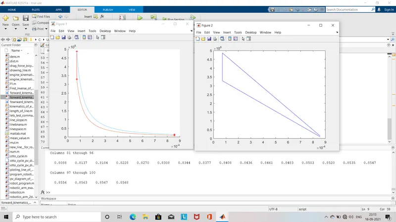
figure(1)                            % figure to show the correct otto cycle
hold on                              % hold all the plots
plot(V1,P1,'*','color','r')          % plot coordinates of state 1
plot(V_compression, P_compression)   % plotting the trace of Volume and pressure during compression

plot(V2,P2,'*','color','r')          % plot coordinates of state 2
plot( [V2,V3],[P2,P3],'color','r')   % join the state 2 and 3 by straight line

plot(V3,P3,'*','color','r')          % plot coordinates of state 3
plot(V_expansion, P_expansion)       % plotting the trace of volume and pressure during expansion
plot(V4,P4,'*','color','r')          % plot coordinates of state 4
plot([V4,V1],[P4,P1])                % join the state 4 and 1 by straight line

%plotting of another straight line otto cycle for comparison
figure(2)                                     % figure to show the wrong otto cycle
plot([V1 V2 V3 V4],[P1,P2,P3,P4],'color','b') % join all the coordinates of states by straight line

%calculation of the thermal efficiency of the engine

eff_term=cr^(gamma-1)      % term  to store the value of cr^(gamma-1)
therm_eff=1-(1/eff_term)   % thermal efficiency of engine


%% errors faced and how did they overcome

%error 1: unrecognized variable or function 'v_comprseesion'
%solution_1: 'V_compression' is written by replacing  'v_comprseesion'

%error 2: expansion adiabatic graph not drawn
%solution 2: in line 65, 'plot(V_compression, P_compression)' is replaced
                                    %by plot(V_expansion, P_expansion)

%error 3: incorrect dimension for raising  matrix to a power
%solution 3:in kinematics_of_engine , line 20, element wise operator was put


%errors graphs and output graphs are attached