Project 2 - Rankine cycle Simulator
AIM: To create the Rankine cycle simulator and to find out the thermodynamic properties of each state.
OBJECTIVE:
- Create a Rankine Cycle Simulator using OCTAVE/MATLAB.
- Calculation of the state points of the Rankine Cycle based on user inputs.
- Plot the corresponding T-s and h-s plots for the given set of inputs.
- Rankine cycle is a thermodynamic cycle which converts heat into mechanical energy—which usually gets transformed into electricity by electrical generator.
- It is the process widely used by power plants such as coal fired power plants or nuclear reactors. In this mechanism, a fuel is used to produce heat within a boiler, converting water into steam which then expands through a turbine producing useful work. This process was developed in 1859 by Scottish engineer William J.M. Rankine.
Fig 1: Basic picture of rankine vapour cycle
- Different processess involved in the rankine vapour cycle are given below
- Isentropic Expansion (1-2): The vapor is expanded in the turbine, thus producing work which may be converted to electricity.
- Isobaric Heat Rejection(2-3): The vapor-liquid mixture leaving the turbine is condensed at low pressure, usually in a surface condenser using cooling water.
- Isentropic Compression(3-4): The pressure of the condensate is raised in the feed pump.
- Isobaric Heat Transfer(4-1): High pressure liquid enters the boiler from the feed pump and is heated to the saturation temperature . Further addition of energy causes evaporation of the liquid until it is fully converted to saturated steam.
What is Isentropic process?
An Isentropic is a thermodynamic process in which the entropy of the fluid or gas remains constant.
What is isobaric process?
An Isobaric process is a thermodynamic process in which pressure of the fluid or gas remains constant
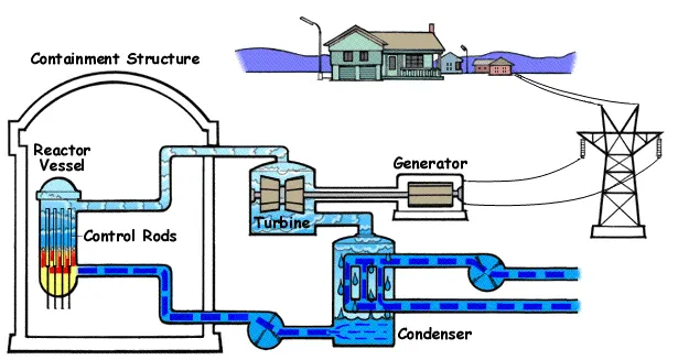
Fig 2: Annimated chart to show the working of rankine cycle
Governing equations
1.Turbine work
WT=h1-h2
2.Pump work
Wp=h4-h3
3.Net work done
Wnet=WT - Wp
4.Thermal efficiency = Wnet/(h1-h4)
5.Back Work Ratio (BWR)
BWR=Wp/WT
6.Specific steam conductivity (S.S.C)
S.S.C = 3600/WT
clear all
close all
clc

% displaying the all the process in their respective devices
disp ('-----------------------RANKINE CYCLE STIMULATOR------------------------')
disp('1-2 is isentropic expansion in turbine')
disp('2-3 is const pressure heat rejection by condenser')
disp('3-4 is isentropic compression by feed pump')
disp('4-1 is const pressure heat addition  by boiler')

% asking the user to input the details
p1=input('enter the pressure at inlet of turbine (in bar): ');             % input inlet turbine pressure
t1=input('enter the temperature at inlet of turbine (in degree celcius: ');% input the inlet turbine temperature
p2=input('enter the pressure at inlet of condenser: ');                    % input the inlet condenser pressure


% calculation of all states

 %state 1
 h1=XSteam('h_pt',p1,t1);   % enthalpy at press p1 and temp t1.
 s1=XSteam('s_pt',p1,t1);   % entropy at press p1 and temp t1.

 % state 2
 s2=s1;                     % isentropic process
 s_l2=XSteam('sL_p',p2);    % entropy at liquid curve at pressure p2
 s_g2=XSteam('sV_p',p2);    % entropy at gas curve at pressure at p2
 h_l2=XSteam('hL_p',p2);    % enthalpy on liquid curve at pressure p2
 h_g2=XSteam('hV_p',p2);    % enthalpy on gas curve at pressure p2
 x=(s1-s_l2)/(s_g2-s_l2);    % calculating the dryness fraction by using s1=s2
 h2=h_l2 + x*(h_g2-h_l2);   % calculating the enthalpy at state 2
 t2=XSteam('T_hs',h2,s2);   % temperature at state 2
 T_sat2 = XSteam('Tsat_p',p2); % saturation temperature at p2

 % At state point 3
 p3=p2;                        % isobaric process so p3=p2
 t3=t2;                        % temperature at state 2 and 3 are same
 h3=XSteam('hL_T',t3);         % saturated liquid enthalpy at state 3
 s3= XSteam('sL_T',t3);        % saturated liquid entropy at state 3

 % state 4
 p4=p1;                        % isobaric process
 s4=s3;                        % isentropic process
 t4=XSteam('T_ps',p4,s4);      % temperature at state 4
 h4=XSteam('H_ps',p4,s4);      % enthalpy at state 4

 % state 5
 t5=XSteam('Tsat_p',p1);       % state 5 temperature
 t6=t5;                        % state 6 temperature
 s5=XSteam('sL_p',p1);         % state 5 saturated liquid entropy at p1
 s6=XSteam('sV_p',p1);         % state 6 saturated vapour entropy at p1
 h5=XSteam('hL_p',p1);         % state 5 saturated liquid enthalpy at p1
 h6=XSteam('hV_p',p1);         % state 6 saturated vapour enthalpy at p1

% calculation of work, back work ratio, specific steam condcuctivity and efficiency
Turb_work= h1-h2;                    % turbine work(expansion)
pump_work= h4-h3;                    % work done by pump
net_work=Turb_work-pump_work;        % net work done by rankine cycle
heat_add=h1-h4;                      % heat addition in boiler
eff=(net_work/heat_add)*100;         % efficiency of rankine cycle

back_work_ratio=pump_work/Turb_work; % back work ratio by  rankine
sp_steam_cd= 3600/Turb_work;         % specific steam conductivity


% plotting the results
fprintf('\n\n')                                % skip the 2 lines
fprintf(' ------------------------------RESULTS------------------------------\n')
fprintf('at state point 1 \n')                 % display  'at state point 1' line
fprintf('P1 is : %.2f Bar \n',p1)              % display the inlet pressure of turbine
fprintf('T1 is : %.2f in Deg celcius \n',t1)   % display the inlet temperature of turbine
fprintf('H1 is : %.2f in KJ/kg \n', h1)        % displayy the enthalpy at state 1
fprintf('S1 is : %.2f in KJ/kgK \n', s1)       % display the entropy of state 1
fprintf('\n\n')                                % skip the 2 lines

fprintf('At state point 2 \n')                 % display 'at state point 2'line
fprintf('P2 is : %.2f Bar \n',p2)              % display the inlet pressure of condenser
fprintf('T2 is : %.2f Deg Celcius \n',t2)      % display the inlet temperature of condenser
fprintf('H2 is : %.2f KJ/Kg \n',h2)            % displayy the enthalpy at state 2
fprintf('S2 is : %.2f KJ/KgK \n',s2)           % display the entropy of state 2
fprintf('X2 is : %.2f \n',x)                   % display the  dryness fraction at 2
fprintf('\n\n')                                % skip the 2 lines

disp('At state point 3 ')                      % display 'at state point 3' line
fprintf('P3 is : %.2f Bar \n',p3)              % display the inlet pressure of pump
fprintf('T3 is : %.2f Deg Celcius \n',t3)      % display the inlet temperature of pump
fprintf('H3 is : %.2f KJ/Kg \n',h3)            % display the enthalpy at state 3
fprintf('S3 is : %.2f KJ/KgK \n',s3)           % display the entropy at state 3
fprintf('\n\n')                                % skip the 2 lines


disp('At state point 4 ')                      % display 'at state point 3' line
fprintf('P4 is : %.2f Bar \n',p4)              % display the inlet pressure of boiler
fprintf('T4 is : %.2f Deg Celcius \n',t4)      % display the output temperature of boiler
fprintf('H4 is : %.2f KJ/Kg \n',h4)            % display the enthalpy at state 4
fprintf('S4 is : %.2f KJ/KgK \n',s4)           % display the entropy at state 4
fprintf('\n\n')                                % skip 2 lines

fprintf('Turbine work : %.2f KJ/Kg \n',Turb_work)  % print the turbine work
fprintf('pump work : %.2f KJ/Kg \n',pump_work)     % print the pump work
fprintf('NET work : %.2f KJ/Kg \n',net_work)       % print the net work done by cycle
fprintf('\n\n')                                    % skip 2 lines

fprintf('thermal efficiency : %.2f \n ',eff)                       % printing the thermal efficiency
fprintf('specific steam conductivity : %f Kg/KWh \n',sp_steam_cd)  % printing  the specific steam conductivity
fprintf('back work ratio : %f \n',back_work_ratio)                 % printing the back work ratio
fprintf('\n\n')                                                    % skip 2 lines


%plotting the graphs
subplot(1,2,1)                                                        % plotting the subplot of T-S diagram
 plot([s1 s2 s3 s4 s5 s6 s1],[t1 t2 t3 t4 t5 t6 t1],'linewidth',1.5)  % joining the states using lines
 hold on                                                              % retain the current plot

% plotting the dome of rankine cycle
temp_curve=linspace(0,400,900);                      % plotting the curve for T-S diagram
    for i= 1:length(temp_curve)                      % loop used to plot each point of curve
     s_l(i)=XSteam('sL_T',temp_curve(i));            % entropy for a saturated liquid curve
     s_v(i)=XSteam('sV_T',temp_curve(i));            % entropy for a saturated gas curve
     h_l(i)=XSteam('hL_T',temp_curve(i));            % enthalpy for saturated liquid curve
     h_v(i)=XSteam('hV_T',temp_curve(i));            % enthalpy for saturated gas curve
    end                                              % terminating the 'for loop'

plot(s_l,temp_curve,'linewidth',2,'color','g')                                            % plotting the liquid saturation curve
plot(s_v,temp_curve,'linewidth',2,'color','g')                                            % plotiing the gas saturation curve
text(s1,t1,'1','fontsize',15)                                                             % naming the state 1 as '1'
text(s2,t2,'2','fontsize',15)                                                             % naming the state 2 as '2'
text(s3,t3,'3','fontsize',15,'HorizontalAlignment','right','VerticalAlignment','top')     % naming the state 3 as '3' with allignments
text(s4,t4,'4','fontsize',15,'HorizontalAlignment','right','VerticalAlignment','bottom')  % naming the state 4 as '4' with allignments
text(s5,t5,'5','fontsize',15)                                                             % naming the state 5 as '5'
text(s6,t6,'6','fontsize',15)                                                             % naming the state 6 as '6'
title('T-S Diagram')                                                                      % title of the subplot
xlabel('Entropy (in KJ/KgK)')                                                             % naming x axis as entropy (in KJ/KgK)
ylabel('Temperature (in degree Celcius)')                                                 % naming y axis as Temperature (in degree Celcius)

 % plotting H-S diagram
 subplot(1,2,2)                                                                           % creating sublot for H-S diagram
 plot([s1 s2 s3 s4 s1],[h1 h2 h3 h4 h1],'linewidth',2)                                    % plotting the lines joining the states
 hold on                                                                                  % retaining the plot
 plot(s_v,h_v,"Color",'r','LineWidth',2)                                                  % plotting the vapor saturation curve
 plot(s_l,h_l,'Color','r','LineWidth',2)                                                  % plotting the liquid saturation curve
 % plotting the liquid saturation curve
 title('H-S Diagram')                                                                     % Title of the subplot
 xlabel('Entropy (in KJ/KgK)')                                                            % naming x axis as 'Entropy (in KJ/KgK)
 ylabel('Enthalpy (in KJ/Kg)')                                                            % naming y axis as 'Enthalpy (in KJ/Kg)
RESULTS
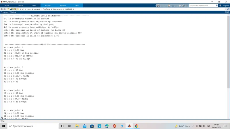
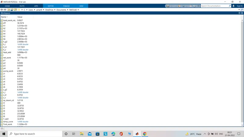
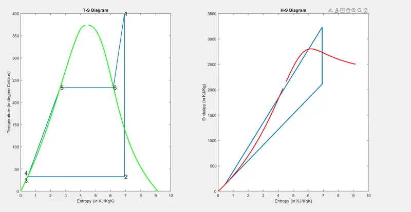
OUTPUT GRAPHS OBTAINED
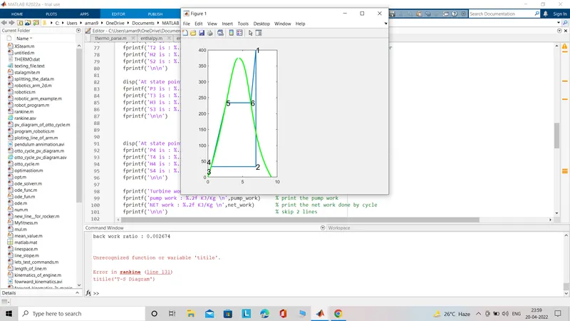
ERROR FACED
- Unrecognized variable 'titile' is found - it is corrected by corrrecting the spelling
REFERENCE