Week 4.1 - Genetic Algorithm

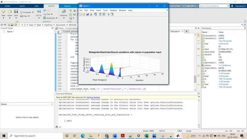
Time Results in seconds:

1. Optimized_Time_Study_after_reducing_area_and_Population =1.8944

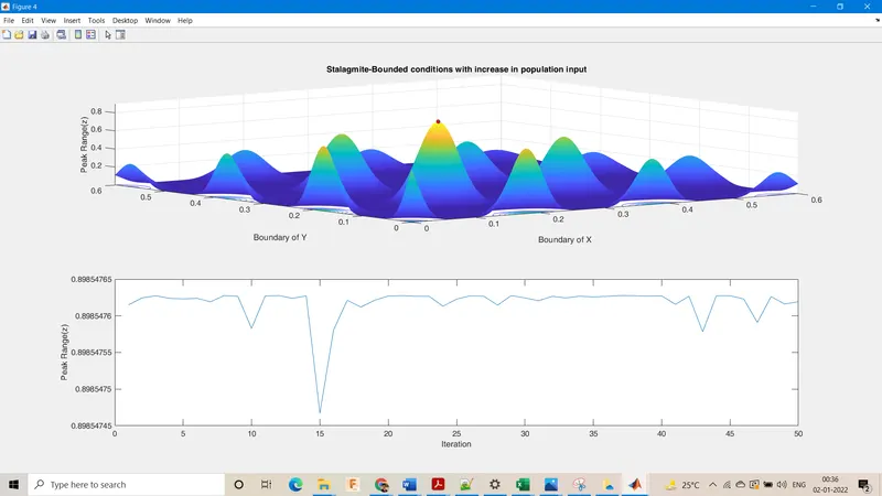
2. Single_Optimized_Time_Study =8.9171

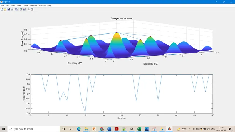
3. Calculation_time_for_bounded_data =2.9535

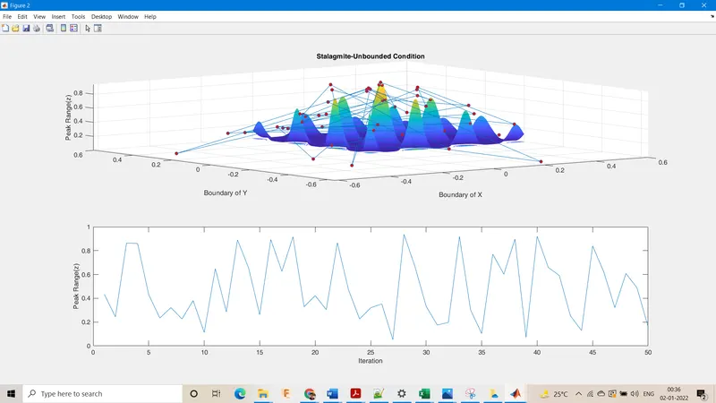
4. Calculation_time =3.3004

Report

1. Set the values of x & y as inputs.

2. Created a 2D meshgrid using x & y.

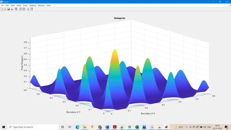
3. Created the stalagmite function using x & y as input vectors.

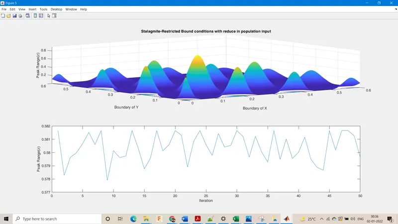
4. Created various figures using the stalagmite function based on various conditions like restricted bound conditions with reducing population, bounded condition with increase inpopulation etc.

Errors:

1. Used subplot(2,1,2) instead of subplot (2,1,1) in figure 5

ans: Corrected it to subplot(2,1,1).

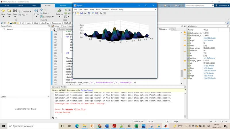
2. Mispelled shading in figure 5 as shding

ans: corrected it to shading.

Concept of Genetic Algorithm:

1. Genetic Algorith is a method of solving constrained & unconstrained optimization problems.

2. This is based on natural selection method

3. GA repeatedly modifies a population of individual solutions.

4. It can generate high quality of solutions to optimization & search problems using biological concepts like mutation, crossover & selection.

%GA
clear all
close all
clc

%set boundaries
x=linspace(0,0.6,150);
y=linspace(0,0.6,150);
iteration=50;

%2D Matrix
[xx yy]=meshgrid(x,y);

%stalagmite func
for i=1:length(xx)
    for j=1:length(yy)
        input_vector(1)=xx(i,j);
        input_vector(2)=yy(i,j);
        f(i,j)=stalagmite(input_vector);
    end
end
figure(1)
surfc(xx,yy,-f)
shading interp
title('Stalagmite')
xlabel('Boundary of X')
ylabel('Boundary of Y')
zlabel('Peak Range(z)')
%%
tic

%CASE 1: Stat behaviour of genetic algo
for i=1:iteration
    [input,Fopt(i)]=ga(@stalagmite,2);
    Xopt(i)=input(1);
    Yopt(i)=input(2);
end

figure(2)
subplot(2,1,1)
surfc(xx,yy,-f)
hold on
title('Stalagmite-Unbounded Condition')
xlabel('Boundary of X')
ylabel('Boundary of Y')
zlabel('Peak Range(z)')
shading interp
plot3(Xopt,Yopt,-Fopt,'o-','markerfacecolor','r','markersize',5)
subplot(2,1,2)
plot(-Fopt)
xlabel('Iteration')
ylabel('Peak Range(z)')
Calculation_time=toc
%%

tic
%case 2:Stat behaviour in bounded region
for i=1:iteration
    lb=[0,0];
    ub=[0.6,0.6];
    [input,Fopt(i)]=ga(@stalagmite,2,[],[],[],[],lb,ub);
    Xopt(i)=input(1);
    Yopt(i)=input(2);
end

figure(3)
subplot(2,1,1)
surfc(xx,yy,-f)
shading interp
title('Stalagmite-Bounded')
xlabel('Boundary of X')
ylabel('Boundary of Y')
zlabel('Peak Range(z)')
hold on
plot3(Xopt,Yopt,-Fopt,'o-','markerfacecolor','r','markersize',5)
subplot(2,1,2)
plot(-Fopt)
xlabel('Iteration')
ylabel('Peak Range(z)')
Calculation_time_for_bounded_data=toc
%%
tic
%case 3:increasing input of population
options=optimoptions('ga','populationsize',215)
for i=1:iteration
    lb=[0,0];
    ub=[0.6,0.6];
    [input,Fopt(i)]=ga(@stalagmite,2,[],[],[],[],lb,ub,[],options);
    Xopt(i)=input(1);
    Yopt(i)=input(2);
end

figure(4)
subplot(2,1,1)
surfc(xx,yy,-f)
shading interp
title('Stalagmite-Bounded conditions with increase in population input')
xlabel('Boundary of X')
ylabel('Boundary of Y')
zlabel('Peak Range(z)')
hold on
plot3(Xopt,Yopt,-Fopt,'o-','markerfacecolor','r','markersize',5)
subplot(2,1,2)
plot(-Fopt)
xlabel('Iteration')
ylabel('Peak Range(z)')
Single_Optimized_Time_Study=toc
%%

tic
%case 4:Increase input of population & restrict bounded condition
options=optimoptions('ga','populationsize',9)
for i=1:iteration
    lb=[0,0];
    ub=[0.1,0.1];
    [input,Fopt(i)]=ga(@stalagmite,2,[],[],[],[],lb,ub,[],options);
    Xopt(i)=input(1);
    Yopt(i)=input(2);
end

figure(5)
subplot(2,1,1)
surfc(xx,yy,-f)
shading interp
title('Stalagmite-Restricted Bound conditions with reduce in population input')
xlabel('Boundary of X')
ylabel('Boundary of Y')
zlabel('Peak Range(z)')
hold on
plot3(Xopt,Yopt,-Fopt,'o-','markerfacecolor','r','markersize',5)
subplot(2,1,2)
plot(-Fopt)
xlabel('Iteration')
ylabel('Peak Range(z)')
Optimized_Time_Study_after_reducing_area_and_Population=toc


%function
function [f]=stalagmite(input_vector)
%f(x,y)=f1x,f2x,f1y,f2y
x=input_vector(1);
y=input_vector(2);
f1x=(sin(5.1*pi*x+5))^6;
f1y=(sin(5.1*pi*y+5))^6;
f2x=exp(-4*log(2)*((x-0.0667)^2)/0.64);
f2y=exp(-4*log(2)*((y-0.0667)^2)/0.64);
f=-(f1x*f1y*f2x*f2y);
end