Project 2 - Rankine cycle Simulator

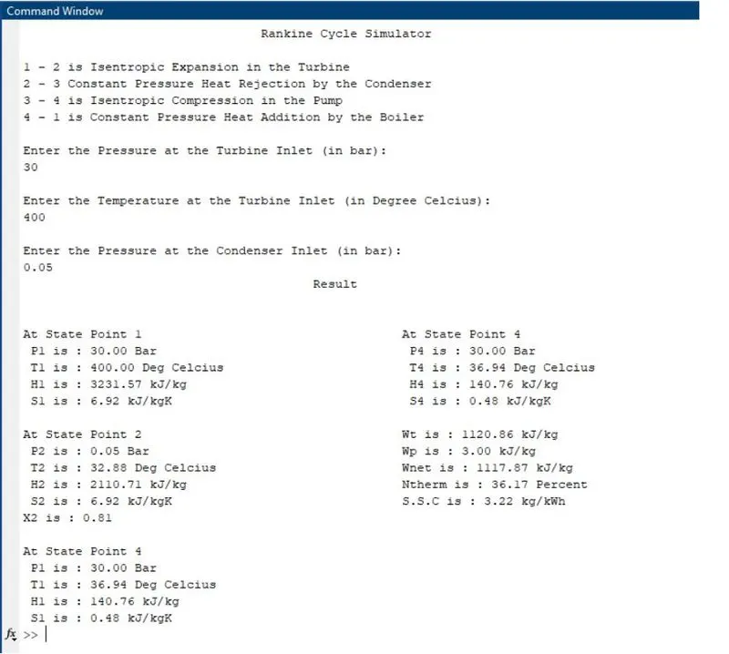
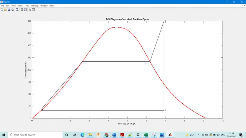
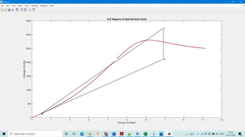
Report:

1. Take inputs of pressures & temperature from users.

2. get enthalpy & entropy from xSteam file.

3. Get condenser,pump, & boiler inlet conditions using XSteam.

4. Calculate work done using given formula

5. calculate heat added, thermal efficiency & specific steam consumption.

6. plot graphs of H-S & T-S.

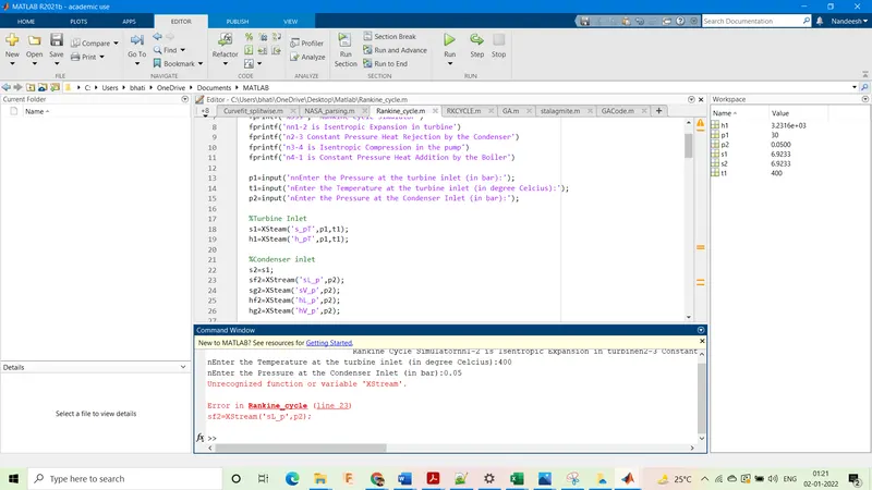
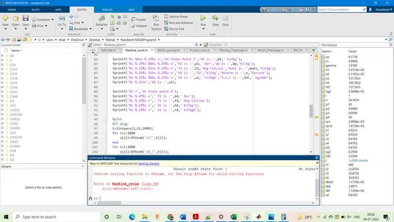
Errors:

1. Wrote XStream instead of XSteam

ans: Corrected it to XStream.

2. Typed sLT instead of sL_T

ans:Corrected as sL_T.

Theory:

The Rankine cycle or Rankine Vapor Cycle is the process widely used by power plants such as coal-fired power plants or nuclear reactors. In this mechanism, a fuel is used to produce heat within a boiler, converting water into steam which then expands through a turbine producing useful work. This process was developed in 1859 by Scottish engineer William J.M. Rankine. This is a thermodynamic cycle that converts heat into mechanical energy, which usually gets transformed into electricity by electrical generation.

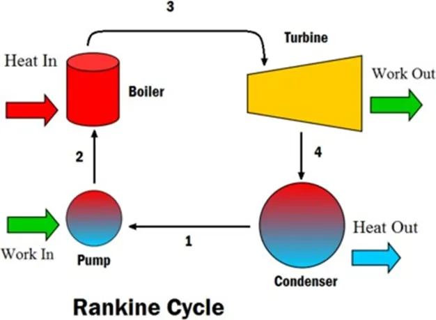
Pump: Compression of the fluid to high pressure using a pump.

Boiler: The compressed fluid is heated to the final temperature.

Turbine: Expansion of the vapor in the turbine.

Condenser: Condensation of the vapor in the condenser.

The efficiency of the Rankine cycle is limited by the high heat of vaporization by the fluid. The fluid must be cycled through and reused constantly, therefore, water is the most practical fluid for this cycle. This is not why many power plants are located near a body of water—that's for the waste heat.

As the water condenses in the condenser, waste-heat is given off in the form of water vapor—which can be seen billowing from a plant's cooling towers. This waste heat is necessary for any thermodynamic cycle. Due to this condensation step, the pressure at the turbine outlet is lowered. This means the pump requires less work to compress the water—resulting in higher overall efficiencies.

Isobaric Heat Transfer or Constant Pressure heat addition in a Boiler

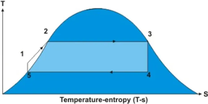
The boiler is a large heat exchanger where heat liberating fuel like coal, lignite, or oil transfers the heat indirectly to water at constant pressure. Water enters the steam boiler from the boiler feed pump as a compressed liquid at state-1 and is heated to the saturation temperature as shown in the T-s diagram as state-3.

The energy balance in the boiler is or energy added in a steam generator,

qin= h3-h1

Isentropic Expansion in a Turbine

Vapor from the boiler outlet enters the turbine at state 3, where it expands isentropically over the turbine fixed and moving blade to produce work done in the form of mechanical rotation of the turbine shaft, which is connected to the electrical generator.

Work delivered by the turbine (Neglecting heat transfer with the surroundings)

Wturbine out= h3-h4

Isobaric Heat Rejection or Constant Pressure heat rejection in a Condenser

At state-4, vapor enters the condenser. The change of phase occurs as vapor is condensed to liquid at constant-pressure in the condenser by transferring the steam’s heat to the circulating water flow through the tubes of the condenser. Change of phase occurs in the condenser, and the working fluid leaving the condenser is in a liquid state and marked as point 5. Energy rejected in the condenser, qout= h4-h5

Isentropic Compression in a Pump

Water exits the condenser at state 5 and enters the pump. This pump raises the pressure of the water by imparting work during the processes. In units of smaller size and low specific volume, this small work can be neglected compared to the work-output of a steam turbine.

Work was done on the pump per kg of water, W51= h5-h1.

Efficiency=(qin-qout)/qin=Wnet/qin.

%Rankine Cycle simulator
clear all
close all
clc

%Input
fprintf('%55s', 'Rankine Cycle Simulator')
fprintf('1-2 is Isentropic Expansion in turbine')
fprintf('2-3 Constant Pressure Heat Rejection by the Condenser')
fprintf('3-4 is Isentropic Compression in the pump')
fprintf('4-1 is Constant Pressure Heat Addition by the Boiler')

p1=input('Enter the Pressure at the turbine inlet (in bar):');
t1=input('Enter the Temperature at the turbine inlet (in degree Celcius):');
p2=input('Enter the Pressure at the Condenser Inlet (in bar):');

%Turbine Inlet
s1=XSteam('s_pT',p1,t1);
h1=XSteam('h_pT',p1,t1);

%Condenser inlet
s2=s1;
sf2=XSteam('sL_p',p2);
sg2=XSteam('sV_p',p2);
hf2=XSteam('hL_p',p2);
hg2=XSteam('hV_p',p2);

%Determining Dryness fraction
if(s2<=sg2)
    x2=((s2-sf2)/(sg2-sf2));
else
x2=1;
end
h2=hf2+(x2*(hg2-hf2));

%pump inlet
p3=p2;
t3=XSteam('Tsat_p',p3);
s3=XSteam('sL_p',p3);
h3=XSteam('hL_p',p3);
t2=t3;

%Boiler Inlet
p4=p1;
s4=s3;
h4=XSteam('h_ps',p4,s4);
cp=XSteam('Cp_ps',p4,s4);
cv=XSteam('Cv_ps',p4,s4);

%determine gamma
gamma=(cp/cv);
t4=(t3*((p3/p4)^((1-gamma)/gamma)));

%work done
%turbine
Wt=h1-h2;
%pump
Wp=h4-h3;
%Net
Wnet=Wt-Wp;

%heat added
%boiler
qin=h1-h4;
%condenser
qout=h2-h3;

%Theraml efficiency
n=(Wnet/qin)*100;

%Specific Stream Consumption
SSC=(3600/Wnet);

%Result
fprintf('%45s nnn','Result');
fprintf('%s %50s n','At State Point 1','At State Point 4');
fprintf('%s %.2f%s %40s %.2f%s n',' P1 is :',p1,' Bar',' P4 is:',p4,' Bar');
fprintf('%s %.2f%s %31s %.2f%s n',' T1 is :',t1,'Deg Celcius','T4 is :',t4,' Deg Celcius');
fprintf('%s %.2f%s %36s %.2f%s n',' H1 is :',h1,'KJ/kg','H4 is :',h4,' KJ/kg');
fprintf('%s %.2f%s %38s %.2f%s n', 'S1 is :',s1,' kJ/kgK',' S4 is :',s4,' kJ/kgK');

fprintf('%s %41s %.2f%s n','At State Point 2','Wt is :',Wt,' kJ/kg');
fprintf('%s %.2f%s %40s %.2f%s n','P2 is :',p2,' Bar','Wp is :',Wp,'kJ/kg');
fprintf('%s %.2f%s %33s %.2f%s n','T2 is :',t2,'Deg Celcius','Wnet is :',Wnet,'KJ/kg');
fprintf('%s %.2f%s %39s %.2f%s n','H2 is :','h2','kJ/kg','Ntherm is :',n,'Percent');
fprintf('%s %.2f%s %40s %.2f%s n','S2 is :',s2,' KJ/kgK','S.S.C is :',SSC,' kg/KWh');
fprintf('%s %.2fnn','X2 is :',x2);

fprintf('%s n','At State point 4');
fprintf('%s %.2f%s n',' P1 is :',p4,' Bar');
fprintf('%s %.2f%s n',' T1 is :',t4,' Deg Celcius');
fprintf('%s %.2f%s n',' H1 is :',h4,' kJ/kg');
fprintf('%s %.2f%s n',' S1 is :',s4,' kJ/kgK');

%plot
%TS diag
t=linspace(1,t1,2000);
for i=1:2000
    sl(i)=XSteam('sL_T',t(i));
end
for i=1:2000
    sv(i)=XSteam('sV_T',t(i));
end
figure(1)
plot(sl,t,'-.r','LineWidth',2)
hold on
plot(sv,t,'-.r','LineWidth',2)
%1-2 State
plot([s1 s2],[t1 t2],'k','LineWidth',1)
%2-3 State
plot([s2 s3],[t2 t3],'k','LineWidth',1)
%3-4 State
plot([s3 s4],[t3 t4],'k','LineWidth',1)
%4-1 State
tp=XSteam('TSat_p',p4);
sp=XSteam('sL_T',tp);
tq=tp;
sq=XSteam('sV_T',tq);
plot([s4,sp],[t4,tp],'k','LineWidth',1)
plot([sp,sq],[tp,tq],'k','LineWidth',1)
plot([sq,s1],[tq,t1],'k','LineWidth',1)
text(s1,t1,' 1');
text(s2,t2,' 2');
text(s3,t3,' 3');
text(s4,t4,' 4');

%PV diag
for i=1:2000
    hl(i)= XSteam('hL_T',t(i));
end
for i=1:2000
    hv(i)=XSteam('hV_T',t(i));
end
figure(2)
plot(sl,hl,'-.r','LineWidth',2)
hold on
plot(sv,hv,'-.r','LineWidth',2)

%1-2 State
plot([s1 s2],[h1 h2],'k','LineWidth',1)
%2-3 State
plot([s2 s3],[h2 h3],'k','LineWidth',1)
%3-4
plot([s3 s4],[h3 h4],'k','LineWidth',1)
%4-1
plot([s4 s1],[h4 h1],'k','LineWidth',1)
text(s1,h1,' 1');
text(s2,h2,' 2');
text(s3,h3,' 3');
text(s4,h4,' 4');