Week 4.1 - Genetic Algorithm
Aim:
- Write a code in MATLAB to optimise the stalagmite function and find the global maxima of the function.
Optimization:
The activity of enhancing system capabilities and integration of subsystem elements to the extent that all components operate at or above user expectations. In other words an act, process, or methodology of making something (such as a design, system, or decision) as fully perfect, functional, or effective as possible specifically : the mathematical procedures (such as finding the maximum of a function) involved in this.
Stalagmite Function:
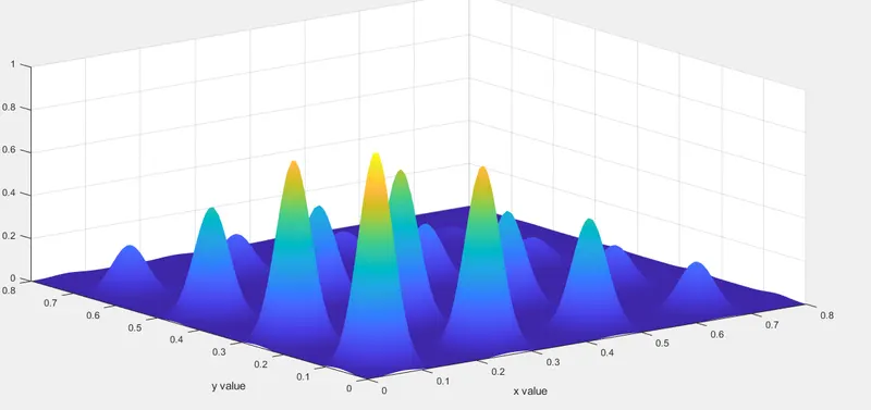
Stalagmites have thicker proportions and grow up on the bottom of a cavern from the same drip-water source, the mineral from which is deposited after the water droplet falls across the open space in the rock. Not every stalactite has a complementary stalagmite, and many of the latter may have no stalactite above them. Where the paired relation exists, however, continual elongation of one or both may eventually result in a junction and the formation of a column.
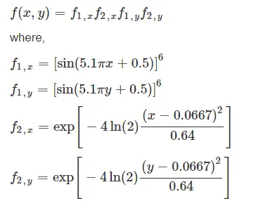
Stalagmite function derived by
Genetic Algorithm:
A genetic algorithm is a search heuristic that is inspired by Charles Darwin’s theory of natural evolution. This algorithm reflects the process of natural selection where the fittest individuals are selected for reproduction in order to produce offspring of the next generation.
The genetic algorithm is a method for solving both constrained and unconstrained optimization problems that is based on natural selection, the process that drives biological evolution. The genetic algorithm repeatedly modifies a population of individual solutions.
Methodology:
Once the genetic representation and the fitness function are defined, a GA proceeds to initialize a population of solutions and then to improve it through repetitive application of the mutation, crossover, inversion and selection operators
Initialization:
The population size depends on the nature of the problem, but typically contains several hundreds or thousands of possible solutions. Often, the initial population is generated randomly, allowing the entire range of possible solutions . Occasionally, the solutions may be "seeded" in areas where optimal solutions are likely to be found.
Selection:
During each successive generation, a portion of the existing population is selected to breed a new generation. Individual solutions are selected through a fitness-based process, where fitter solutions (as measured by a fitness function are typically more likely to be selected. Certain selection methods rate the fitness of each solution and preferentially select the best solutions. Other methods rate only a random sample of the population, as the former process may be very time-consuming.
Mutation:
For each new solution to be produced, a pair of "parent" solutions is selected for breeding from the pool selected previously. By producing a "child" solution using the above methods of crossover and mutation, a new solution is created which typically shares many of the characteristics of its "parents". New parents are selected for each new child, and the process continues until a new population of solutions of appropriate size is generated. Although reproduction methods that are based on the use of two parents are more "biology inspired", some research suggests that more than two "parents" generate higher quality chromosomes.
Heuristics:
In addition to the main operators above, other heuristics may be employed to make the calculation faster or more robust. The speciation heuristic penalizes crossover between candidate solutions that are too similar; this encourages population diversity and helps prevent premature copnvergence to a less optimal solution.
Termination
This generational process is repeated until a termination condition has been reached. Common terminating conditions are:
- A solution is found that satisfies minimum criteria
- Fixed number of generations reached
- Allocated budget (computation time/money) reached
- The highest ranking solution's fitness is reaching or has reached a plateau such that successive iterations no longer produce better results
- Manual inspection
- Combinations of the above
Syntax of GA:
x = ga(fun,nvars,A,b,Aeq,beq,lb,ub,nonlcon)nonlcon. The function nonlcon accepts x and returns vectors C and Ceq, representing the nonlinear inequalities and equalities respectively. ga minimizes the fun such that C(x) ≤ 0 and Ceq(x) = 0. (Set lb=[] and ub=[] if no bounds exist.)
Stalagmite Function:
function [F] =stalagmite(input_vector)

          x = input_vector(1);
          y = input_vector(2);

          f1 = (sin(5.1*pi*x+0.5))^6;
          f2 = (sin(5.1*pi*y+0.5))^6;
          f3 = exp(-4*log(2)*((x-0.0667)^2)/0.64);
          f4 = exp(-4*log(2)*((y-0.0667)^2)/0.64);

          F =  (f1*f2*f3*f4);
end
program explain:
Finding the 'f value create stalagmite function with x,y input. first 'x' takes a input_vector(1),'y' takes a input_vector(2),then substute the value in stalagmite function formula and finally get 'f' value.
Finding Minimum program:
clear all
close all
clc

% defining x,y value

x = linspace(0,0.8,150);
y = linspace(0,0.8,150);

% 2d array

[xx yy] = meshgrid(x,y);

% evalution 0f stalagmite function

for i = 1:length(xx)
    for j= 1:length(yy)

        input_vector(1) = xx(i,j);
        input_vector(2) = yy(i,j);

        f(i,j) = stalagmite(input_vector);
    end
end

figure(1)
surf(xx,yy,f)
xlabel('x value')
ylabel('y value')
shading interp

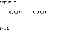
[input,fval] = ga(@stalagmite,2)
program Explain:
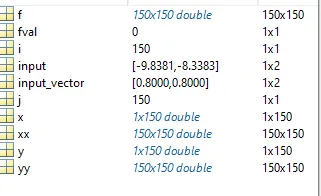
Initially clear,close all,clc- its clear workspce,command as well plot window. Then provide x,y value,then create meshgrid to convert into matrix.,Then write for loop i=length of xx,j = length of yy,Then write the f(i,j) =stalagmite(input_vector); above we write stalagmite function and finally we get ''f'' value after that surf to create 3d plot,give x,y lavel name, shading intrep = stalagmite get smoothet.' ga(@stalamite,2) to get input,fval value..
Output value:
Finding the maximun value:
Finding the global maxima value using staglamite function .
function [F] =stalagmite(input_vector)

          x = input_vector(1);
          y = input_vector(2);

          f1 = (sin(5.1*pi*x+0.5))^6;
          f2 = (sin(5.1*pi*y+0.5))^6;
          f3 = exp(-4*log(2)*((x-0.0667)^2)/0.64);
          f4 = exp(-4*log(2)*((y-0.0667)^2)/0.64);

          F =  -(f1*f2*f3*f4);
end
This above program already explain early and (-) negative sign helps to get maxima value.
Main program:
clear all
close all
clc

% defining x,y value

x = linspace(0,0.6,150);
y = linspace(0,0.6,150)
num_cases = 50;

% 2d array

[xx yy] = meshgrid(x,y);

% evalution 0f stalagmite function

for i = 1:length(xx);
    for j= 1:length(yy);

        input_vector(1) = xx(i,j);
        input_vector(2) = yy(i,j);

        f(i,j) = stalagmite(input_vector);
    end
end

% case1 statical behaviour

tic

for i = 1:num_cases;
    [input, fopt(i)] = ga(@stalagmite,2);
    xopt = input(1);
    yopt = input(2);

end


study1_time = toc

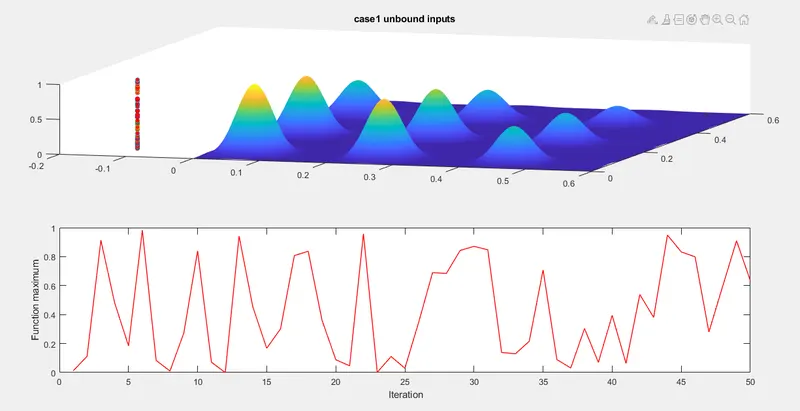
figure(1)
subplot(2,1,1)
hold on
surf(x,y,-f)
shading interp
plot3(xopt,yopt,-fopt,'marker','O','MarkerSize',5,'MarkerFaceColor','r')
title('case1 unbound inputs')
subplot(2,1,2)
plot(-fopt,'LineWidth',1,'Color','r')
xlabel(' Iteration')
ylabel('Function maximum')

% case2 upper and lower bound behaviour

tic

for i = 1:num_cases;
    [input, fopt(i)] = ga(@stalagmite,2,[],[],[],[],[0;0],[1,1]);
    xopt = input(1);
    yopt = input(2);

end


study2_time = toc

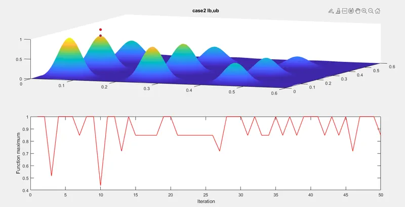
figure(2)
subplot(2,1,1)
hold on
surf(x,y,-f)
shading interp
plot3(xopt,yopt,-fopt,'marker','O','MarkerSize',5,'MarkerFaceColor','r')
title('case2 lb,ub')
subplot(2,1,2)
plot(-fopt,'LineWidth',1,'Color','r')
xlabel(' Iteration')
ylabel('Function maximum')


% case3 ga increse iteration
options = optimoptions('ga');
options = optimoptions(options,'PopulationSize',170);

tic

for i = 1:num_cases;
    [input, fopt(i)] = ga(@stalagmite,2,[],[],[],[],[0;0],[1;1],[],[],options);
    xopt = input(1);
    yopt = input(2);

end


study3_time = toc

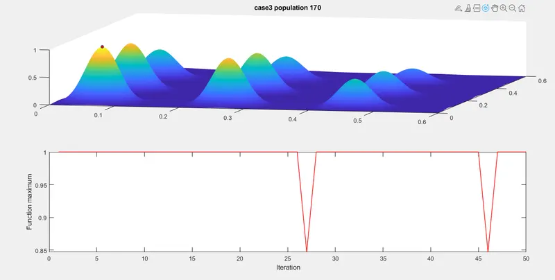
figure(3)
subplot(2,1,1)
hold on
surf(x,y,-f)
shading interp
plot3(xopt,yopt,-fopt,'marker','O','MarkerSize',5,'MarkerFaceColor','r')
title('case3 population 170')
subplot(2,1,2)
plot(-fopt,'LineWidth',1,'Color','r')
xlabel(' Iteration')
ylabel('Function maximum')


% case4 ga increse iteration

options = optimoptions('ga');
options = optimoptions(options,'PopulationSize',300);

tic

for i = 1:num_cases;
    [input, fopt(i)] = ga(@stalagmite,2,[],[],[],[],[0;0],[1;1],[],[],options);
    xopt = input(1);
    yopt = input(2);

end


study4_time = toc

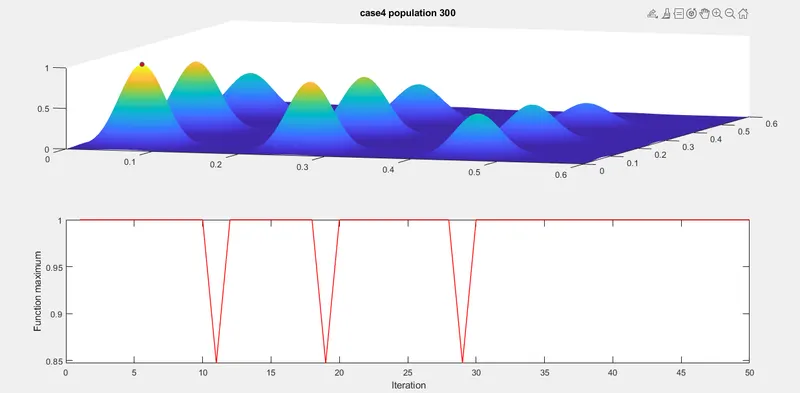
figure(4)
subplot(2,1,1)
hold on
surf(x,y,-f)
shading interp
plot3(xopt,yopt,-fopt,'marker','O','MarkerSize',5,'MarkerFaceColor','r')
title('case4 population 300')
subplot(2,1,2)
plot(-fopt,'LineWidth',1,'Color','r')
xlabel(' Iteration')
ylabel('Function maximum')
Program step wise Explain:
case1:
tic = stop watch start
for i = 1:num_cases; % i =length of num_cases /// num case = 50
[input, fopt(i)] = ga(@stalagmite,2); % stalgmite- function,2 =no fo design variables (fun,nvars)
xopt = input(1); % xopt = input1
yopt = input(2); % yopt = input2
end % finish the foor loop
study1_time = toc % stop watch stop
case2:
In case 2 ga syntex (fun,nvars,Aineq,Bineq,Aeq,Beq,lb,ub)
tic = stop watch start
for i = 1:num_cases; % i =length of num_cases /// num case = 50
[input, fopt(i)] = ga(@stalagmite,2,[],[],[],[],[0;0],[1,1]);
xopt = input(1);
yopt = input(2);
end
Take Aineq =[], Bineq = [], Aeq = [], Beq = [], lb = [], ub = [].
(Set A=[] and b=[] if no linear inequalities exist.)
(Set Aeq=[] and beq=[] if no linear equalities exist.)
(Set lb=[] and ub=[] if no bounds exist.)
(Set nonlcon=[] if no nonlinear constraints exist.)
case3:
options = optimotions('ga')
options = optimotions(options,'populationsize', 170)
IN this method we increasing 'ga' value as take 170 ='ga' ==solver , 'populatiosize'==parametre ,value =200.
for i = 1:num_cases;
[input, fopt(i)] = ga(@stalagmite,2,[],[],[],[],[0;0],[1;1],[],[],options);
xopt = input(1);
yopt = input(2);
end
figure(3) % create figure
subplot(2,1,1) % create subplot(2x1) 1-firstplot
hold on % continue with the last plot
surf(x,y,-f) % surf- creating surface plot(3d)
shading interp % plot to make be smoother
plot3(xopt,yopt,-fopt,'marker','O','MarkerSize',5,'MarkerFaceColor','r') %plot3 ==3d plot
title('case3 population 170') % title
subplot(2,1,2) % subplot(2x1) 2-subplot
plot(-fopt,'LineWidth',1,'Color','r') %plot(fopt value)
xlabel(' Iteration') % xlabel name
ylabel('Function maximum') % ylabel name
Results:
case1(unbounded inputs)
Case2:(lb,ub)
Case 3:(population 170)
Case 4: (population 300)
Sotpping Cretirea:
Some of the most common stopping conditions are: execution time, total number of iterations, non-improving iterations, optimal (lower bound for min, upper bound for max) solution found.
Conclusion:
* using genetic algorithms are used to get minimal and maxima value to be completed sucessfully.