Week 3 - Solving second order ODEs
Aim:
To write the program and simulate the simple pendulum using matlab.
Objective:
1. To write a program and get plot of time,velocity and displacement.
2. Simulation of the simple pendulum.
Introduction:
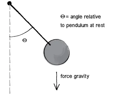
A simple pendulum consists of a ball (point-mass) m hanging from a (massless) string of length L and fixed at a pivot point P. When displaced to an initial angle and released, the pendulum will swing back and forth with periodic motion. By applying Newton's secont law for rotational systems, the equation of motion for the pendulum may be obtained.
Second order differentials equations:
In the second order differential equations have damping co-efficient(b), mass(m), gravity(g), Length(l)
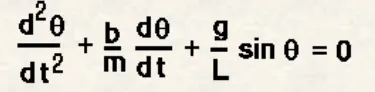
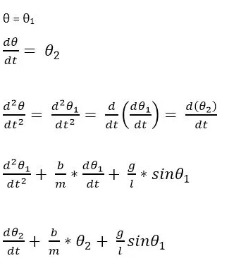
Above the equation is derived as,
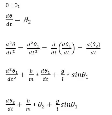
Explanation of problem:
% input
L=1 metre,
m=1 kg,
b=0.05.
g=9.81 m/s2.
% Initial condition
1. angular displacement=0,angular velocity=3 rad/sec at time t=0.
2. motion between 0-20 sec
Matlab program:
clear all                  % clear work space
close all                  % close plot
clc                        % clear command window

% inputs

b = 0.05;                 % b = damping coefficient
g= 9.81;                  % g = gravity
l = 1;                    % l = length
m = 1;                    % m = mass


% initial condition

theta_0 = [0,3];          %displacement = 0, velocity = 3

% time span

t_span = linspace(0,20,500);  % Get random number between (0,20,500)

% solve ode

[t,results] = ode45(@(t,theta) ode_func(t,theta,b,g,l,m), t_span, theta_0);


figure(1)                     % its denoting the first plot
plot(t,results(:,1))          % create plot between(t, results)
hold on                       % hold on is used to continue with the last plot
plot(t,results(:,2))
grid                          % grid enable
xlabel('Time')                % xlabel name
ylabel('Angular displacement vs Angular velocity') %ylabel name
legend('Angular displacement',' Angular velocity')

% Animating the simple pendulum

ct =1

for i = 1:length(results(:,1))  % length of results (500)
    angle = results(i,1);

    x0 = 0;                     % x,y =0
    y0 =0;

    x1 = 1*sin(angle);          % find x1,y1 value
    y1 = -1*cos(angle);

    % plotting

    figure(2)                  % its denote 2nd plot

    plot([-1 1],[0 0],'linewidth',4)  % its only draw line at given value
    axis([-1.5 1.5 -1.5 1.5])          % axis is used to set limit of x,y
    line([x0 x1],[y0 y1],'linewidth',4)
    hold on
    plot(x1,y1,'O','markers',20,'markerfacecolor','r')
    hold off
    pause(0.05);                      % this used to capute the animation
    M(ct) = getframe(gcf);             % get current figure
    ct = ct+1;                         % create advance frame

end
movie(M)
Videofile = VideoWriter('pendulum.avi','Uncompressed AVI');
open(Videofile)
writeVideo(Videofile,M)
close(Videofile)
For loop Explained:
In for loop i =1:length(results(:,1),- (:,1) - column matrix, length of results is(500)
x0 = 0, y0 =0 , === (its fixed point,so xo,yo value are consider as '0')
x1 = 1*sin(angle); ==== l=1 is assumed , x= sin = pendulum is touch in 'y axis'
y1 = -1*cos(angle); ====l=1 is assumed, y = cos = pendulum is not touch in 'x axis'
Function program solved
This function of ode_func(t, theta,b,g,l,m) derive from the program.
function [dtheta_dt] = ode_func(t,theta,b,g,l,m)

theta1 = theta(1);
theta2 = theta(2);

dtheta1_dt = theta2;
dtheta2_dt = -(b/m)*theta2 - (g/l)*sin(theta1);

dtheta_dt = [dtheta1_dt; dtheta2_dt];

end
this program is helps the dependent and independent value.
Error:
1Error : i=1:length(t_span)
over come error: i = length(results(:,1))
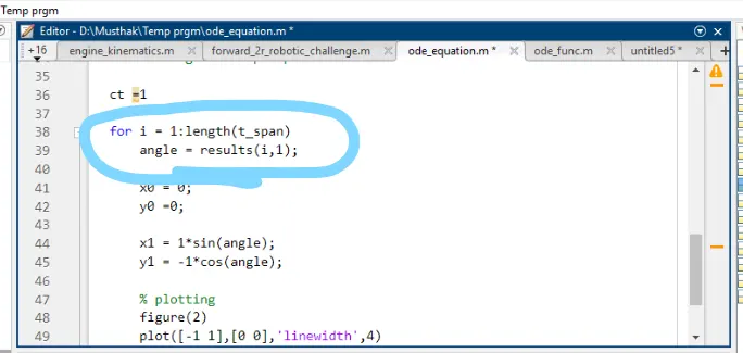
2 Error:
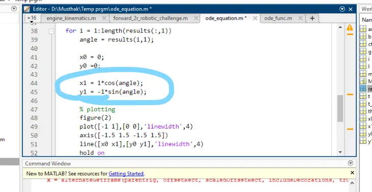
Error:
x1 = 1*cos(angle)
y1 = -1*sin(angle)
Over come error:
x1 = 1*sin(angle)
y1 = -1*cos(angle)
Code and output Explanation:
Output:
The simulate the simple animate the motion of the pendulum is sucessfully completed, all the file attached it.
Code:
clear all % clear work space
close all % close plot
clc % clear command window
% inputs
b = damping coefficient
g = gravity
l = length
m = mass
linspace(0,20,500); % Get random number between (0,20,500)
figure(1)- its explain the time vs Angular displacement &Angular velocity graph
figure (2) - its explain the animation of pendulum
grid - enble grid
xlabel-(x -axis name)
ylabel-(y-axis name)
% Animating the simple pendulum
ct =1 - creating frame
for loop - calculate the multiple value for multilple times.
for i = 1:length(results(:,1)) - % length of results (500)
angle = results(i,1);
x0 = 0; % x,y =0
y0 =0;
x1 = 1*sin(angle); % find x1,y1 value
y1 = -1*cos(angle);
plot([-1 1],[0 0],'linewidth',4) % its only draw line at given value
axis([-1.5 1.5 -1.5 1.5]) % axis is used to set limit of x,y
linewidth - line size
pause(0.05); % this used to capute the animation
M(ct) = getframe(gcf); % get current figure
ct = ct+1; % create advance frame
For loop Explained:
In for loop i =1:length(results(:,1),- (:,1) - column matrix, length of results is(500)
x0 = 0, y0 =0 , === (its fixed point,so xo,yo value are consider as '0')
x1 = 1*sin(angle); ==== l=1 is assumed , x= sin = pendulum is touch in 'y axis'
y1 = -1*cos(angle); ====l=1 is assumed, y = cos = pendulum is not touch in 'x axis'
Solve ode45:
[t,results] = ode45(@(t,theta) ode_func(t,theta,b,g,l,m), t_span, theta_0);
ode45 - used as a matlab program ,ode is fuction of(t,theta)
ode_func - sepreate matlab program(t,theta,l,g,b,m)
t_span - linspace(0,20,500)-(time 0,20 sec ,500 value)
theta_0 - [0,3]- its displacement & velocity value
Function Explanation:
function [dtheta_dt] = ode_func(t,theta,b,g,l,m)
theta1 = theta(1);
theta2 = theta(2);
dtheta1_dt = theta2;
dtheta2_dt = -(b/m)*theta2 - (g/l)*sin(theta1);
dtheta_dt = [dtheta1_dt; dtheta2_dt];
end
Results:
1. plot(Time vs Angular displacement , Angular velocity)
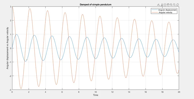
2. plot the animation of simple pendulum:
Conclusion: Finally completed the plot between Time vs Angulardisplacement,Angular velocity and the simulation of simple pendulum.