Week 4.1 - Genetic Algorithm

Genetic Algorithm :

The Genetic algorithm is used for obtaining the high quality of solution for optimization ,search problems , operation research problems by relying on the biologically inspired operation like selection , crossover and the mutation . In GA process the solution candidates for optimization problem are evolved toward better solution

The GA process is carried out in 4 process as

A) Initialization : Initially the population is generated randomly for entire range of possible solution . sometimes the solution is seeded for areas where optimal solution likely to be found .

B) Selection : During the each successive genetation , the portion of the existing generation is selected to breed a new generation . Individually each solution are selected through fittness based process , which check the fitness of each solution and measures the quality new solution .

C) Crossover : The next step is to produce a new generation population through the solution , for each new solution , the "parent" solutions are selected for the bredding from the pool selected previously . In this process the many characters from parents are shared with the new "child" solution .

D) Mutation : Then the mutation is done within the " child " solution for producing the next generation solution , in this process the quality of new generated solution is incresed by mutation process .

E) Termination : It is the final process , the generation process is reapeted until the termination condition has been reached . following are the comman codition for termination :

a) Solution is found that satisfy the minimum criteria

b) Maximum nnumber of generation has reached

c) allocted time reached

d) highest ranking solution is reached

e) combination of above

Syntax

x = ga(fun,nvars) finds a local unconstrained minimum ,x, to the objective function ,fun . nvars is the dimension ( Design variables ) of fun .

1. Program code for optimization of stalagmite function :

clear all
close all
clc

% Defining our search space
x = linspace(0,0.6,100);
y = linspace(0,0.6,100);
num_cases = 50;

%creating the 2D array mesh
[xx yy]=meshgrid(x,y);

for i =1:length(xx)
    for j = 1:length(yy)
        input_vector(1)=xx(i,j);
        input_vector(2)=yy(i,j);
        f(i,j)=stalagmite_func(input_vector);
    end
end

%case1(Unbounded)
tic
for i =1:num_cases                          % for loop will run from 0 to 50(num cases)
    [inputs, fval(i)] =ga(@stalagmite_func,2);
    x_out(i)=inputs(1);
    y_out(i)=inputs(2);
end

case_time = toc;
%plot
figure(1)
subplot(2,1,1);
surfc(xx,yy,-f);
title('case1 Unbounded');
xlabel('x');
ylabel('y');
shading interp;
hold on;
plot3(x_out,y_out,-fval,'marker','O','MarkerSize',6,'markerfacecolor','r');
subplot(2,1,2);
plot(-fval);
xlabel('Number of Iteration');
ylabel('Maximum function value');


% case2 Appling the boundry condition
tic
for i =1:num_cases
    [inputs, fval(i)] =ga(@stalagmite_func,2,[],[],[],[],[0;0],[0.6;0.6]);
    x_out(i)=inputs(1);
    y_out(i)=inputs(2);
end

case_time2 = toc;
%plot
figure(2)
subplot(2,1,1);
surfc(xx,yy,-f);
title('case2', 'Bounded inputs','color','g');
xlabel('x');
ylabel('y');
shading interp;
hold on;
plot3(x_out,y_out,-fval,'marker','O','MarkerSize',6,'markerfacecolor','r');
subplot(2,1,2);
plot(-fval);
xlabel('Number of Iteration');
ylabel('Maximum function value');

% Casa3 incresing the population 
options = optimoptions('ga');
options = optimoptions(options,'PopulationSize',120);

 tic
for i =1:num_cases
    [inputs, fval(i)] =ga(@stalagmite_func,2,[],[],[],[],[0;0],[0.6;0.6],[],[],options);
    x_out(i)=inputs(1);
    y_out(i)=inputs(2);
end

case_time3 = toc;
%plot
figure(3)
subplot(2,1,1);
surfc(xx,yy,-f);
title('case3', 'Increased population','color','g');
xlabel('x');
ylabel('y');
shading interp;
hold on;
plot3(x_out,y_out,-fval,'marker','O','MarkerSize',6,'markerfacecolor','r');
subplot(2,1,2);
plot(-fval);
xlabel('Number of Iteration');
ylabel('Maximum function value');


% Casa4 Increasing population by 250
options = optimoptions('ga');
options = optimoptions(options,'PopulationSize',250);

 tic
for i =1:num_cases
    [inputs, fval(i)] =ga(@stalagmite_func,2,[],[],[],[],[0;0],[0.6;0.6],[],[],options);
    x_out(i)=inputs(1);
    y_out(i)=inputs(2);
end

case_time4 = toc;
%plot
figure(4)
subplot(2,1,1);
surfc(xx,yy,-f);
title('case3', 'Increased population to 250','color','g');
xlabel('x');
ylabel('y');
shading interp;
hold on;
plot3(x_out,y_out,-fval,'marker','O','MarkerSize',6,'markerfacecolor','r');
subplot(2,1,2);
plot(-fval);
xlabel('Number of Iteration');
ylabel('Maximum function value');

% Casa5 Increasing the population to 300
options = optimoptions('ga');
options = optimoptions(options,'PopulationSize',300);

 tic
for i =1:num_cases
    [inputs, fval(i)] =ga(@stalagmite_func,2,[],[],[],[],[0;0],[0.6;0.6],[],[],options);
    x_out(i)=inputs(1);
    y_out(i)=inputs(2);
end

case_time5 = toc;
%plot
figure(5)
subplot(2,1,1);
surfc(xx,yy,-f);
title('case3', 'Increased population to 300','color','g');
xlabel('x');
ylabel('y');
shading interp;
hold on;
plot3(x_out,y_out,-fval,'marker','O','MarkerSize',6,'markerfacecolor','r');
subplot(2,1,2);
plot(-fval);
xlabel('Number of Iteration');
ylabel('Maximum function value');

Expaination Steps:

1. At first randon array of x and y are created by the command : linspace (0,0.6,100) , and number of iterations are provided 50 (i.e. ga will run program for 50 iterations) for which the 2D mesh is created by using the command : meshgrid(x,y) .

2. The for loop is used for assighning values from this array named as the input_vectore which is the input to stalagmite function which is written saperately .

3. Generally the Genetic algorithum process in matlab gives output as global minima , hence i have given the negative sign to output of stalagmite , so that we will get the global maxima as output.

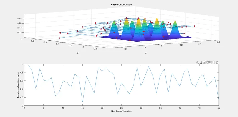
4. In 1st case , we have not defined the boundries and plots are made and here also negative sign is give to get the graph in upward direction.

5. After executing the code just for 1st case , the error is thrown in command window which can be seen in below attached image name ga error , which is overcome by resaving the file by functions name .

5. Tic-Toc command is used to calculate the time required to calculate run time for every case

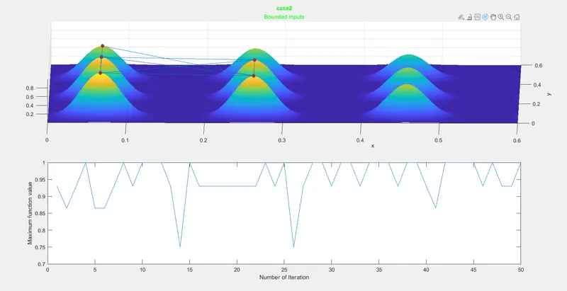
6.In next case i have provided the boundery condition , so we will get more accurate solution for global maxima .

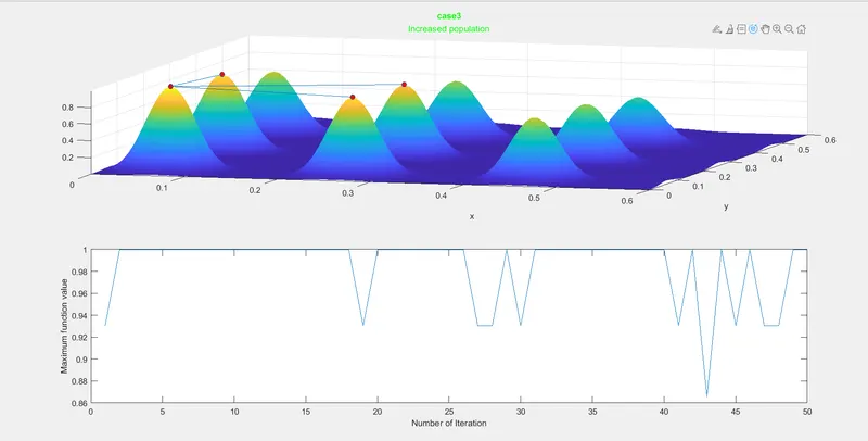
7. For next case i have increased the population

command :

so that solution will approach towards the more accurate and i got the solution in 3 values which is still wasn't accurate .

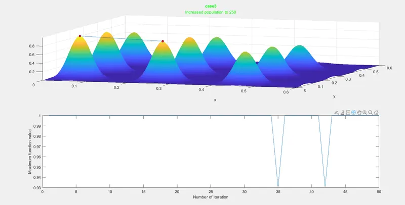
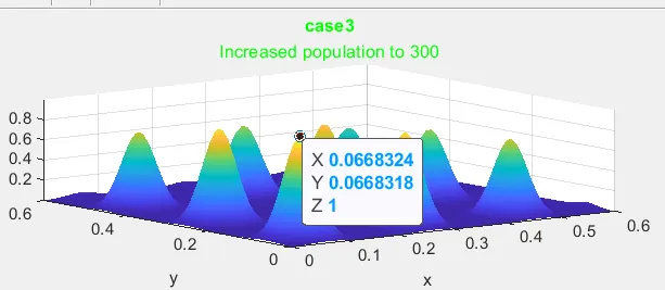
8.For more accurate solution , i have increased the value of population to 300 , this tends to result in more accurate solution for the golbal maxima . and the plots for each case can be seen in below.

Program code for stalagmite function :

 % Creating function for stalagmite 

function [f]= stalagmite_func(input_vector)
% Defining our search space
x = linspace(0,0.6,150);
y = linspace(0,0.6,150);

% converting the Formula into simple term 
% Optimization
term1 = (sin(5.1*pi*input_vector(1) + 0.5)).^6;
term2 = exp(-4*log10(2)*((input_vector(1)-0.0667).^2/0.64));
term3 = (sin(5.1*pi*input_vector(2)+0.5)).^6;
term4 = exp(-4*log10(2)*((input_vector(2)-0.0667).^2/0.64));

% Performing optimization
f1 = term1*term2*term3*term4;
f = -f1;
end

Results :

Case 1 : Unbounded :

Case 2 : Bounded Inputs

Case 3: Increasing the population to 120 :

Case 4: Increasing population to 250 :

Case 5: Increasing population to 300 :

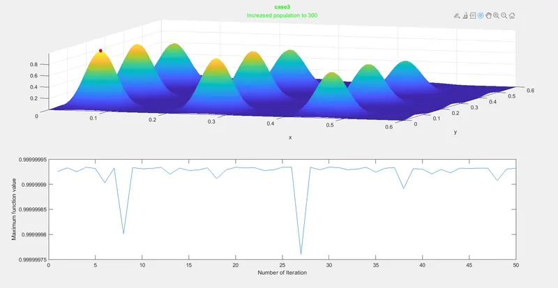
Maximum Value of function for X and Y :

Referance : Wikipedia , https://in.mathworks.com/help/gads/index.html?s_tid=CRUX_lftnav .