Challenge

Week 4.1 - Genetic Algorithm

GGnanasekar Ulaganathan19 Dec 2021

GLOBAL MAXIMA FOR THE STALAGMITE FUNCTION WITH GENETIC ALGORITHM

OBJECTIVE:

To write a MATLAB code to optimise the stalagmite function & determine the global maxima of that function using the genetic algorithms.

Stalagmite:

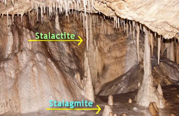
Stalagmite is a type of rock formation rises from the ground by the dripping of the material from the top of the roof. These are generally formed by the calcium carbonate salts from dripping of water from roof of the caves as shown in the below image. This could be also formed by the lava, mud, peat, sand etc., The corresponding formation hanging down from the rook is called the stalactite.

Optimization

Optimization is the process of finding decisions that satisfy the given constraints and meet a specific goal with optimal condition. Constraints could be physical, economical, technical resources, time etc based on the application. Researches are often forced to settle with feasible solutions when using the classic optimization techniques which mostly are the local solutions i.e., sub-optimal solutions. Major problems with the classic optimization techniques are they are entrapped inside the local minima when searching for the global minima & the time duration required increases exponentially with the increase in design variables.

Global optimization algorithm is a procedure which is repeated by comparing various solutions until an optimum solution is arrived. Two major types of global optimization algorithms are listed below

Deterministic algorithms: Use the specific rules for moving from one solution to another.
Stochastic algorithms: Use the probabilistic approach similar to the nature

The genetic algorithm which is a part of the stochastic algorithm solves optimization problems by mimicking the principles of biological evolution, repeatedly modifying a population of individual points. Due to its random nature, the genetic algorithm improves the chances of finding a global solution. They prove to be very efficient and stable in searching for global optimum solutions. it does not require the functions to be differentiable or continuous.

Concept of the genetic algorithm:

Genetic algorithm is part of the evolutionary algorithms which is based on the evolution of life. Genetic algorithm is inspired by the process of the natural selections which are generally used for the optimization & search problems.

Initialization:

The Process starts with the initial set of individuals which are called initial population. The individuals are generally created randomly where each individual is a solution to the problem which is represented by a string of defining characteristics. The defining characteristics are called genes & the string of the genes are referred to the chromosome. Usually, we use binary values for each gene so to make a string of binary numbers to generate the chromosome.

Selection:

The fitness function estimates the fitness scores of the individual based on the ability to compete with other individuals in the same population. Selection is a process where the individuals with higher scores of fitness are chosen as parents for the creation of the next generation.

Population creation for next generation:

The population for the next generation is created based on the combination of the natural selection, Crossover, Mutation.

Crossover: Two of the best fitness scores is chosen as parents and two children are formed by the single, double or multiple crossovers i.e., swapping of the contents of the two parents at the crossover lines. Below is the example of the single point crossover.

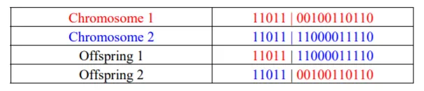
Mutation: To preserve the diversity of the population, few of the genes are modified or mutated to form the new child.
Replace & Accepting: The individuals with lower fitness scores of the previous generation are replaced with the new offspring into the existing population so as to maintain the population size constant.

Revalidation & Stopping criteria:The fitness scores of the new generation are determined and the stopping criteria is checked. If the stopping criteria is not met then the Population creation for next generation is repeated. The stopping criteria could be anhything like number of iterations, improvement in values from previous iterations being lower than the specified target, etc.

Syntax of ga in MATLAB:

Below are the syntax available for the ga in MATLAB

x = ga(fun,nvars)

x = ga(fun,nvars,A,b)

x = ga(fun,nvars,A,b,Aeq,beq)

x = ga(fun,nvars,A,b,Aeq,beq,lb,ub)

x = ga(fun,nvars,A,b,Aeq,beq,lb,ub,nonlcon)

x = ga(fun,nvars,A,b,Aeq,beq,lb,ub,nonlcon,options)

x = ga(fun,nvars,A,b,Aeq,beq,lb,ub,nonlcon,intcon)

x = ga(fun,nvars,A,b,Aeq,beq,lb,ub,nonlcon,intcon,options)

x = ga(problem)

[x,fval] = ga(___)

[x,fval,exitflag,output] = ga(___)

[x,fval,exitflag,output,population,scores] = ga(___)

Where,

fun : objective function

nvars: number of design variable in the objective function

A, b : linear inequalities for the x like A*x <= b, if not applicable [ ],[ ] will be mentioned

Aeq, beq: linear equalities like Aeq*x=beq, if not applicable [ ],[ ] will be mentioned

lb,ub : lower bound & upper bound for the x values which defines the search space ,lb <=x<=ub. Eg lb=[0,0] & ub=[1,1] , if not applicable [ ],[ ] will be mentioned

nonlcon: minimization constraints specified in the function nonlcon (nonlinear constraints). nonlcon accepts x and returns C & Ceq representing the linear inequalities & equalities respectively. ga uses these function to minimize the objective function with the constraint C (x) <=0 & Ceq(x) =0. If not applicable [ ] is mentioned.

options : default optimization parameters replaced by values specified in options. Few of the values which are optimized are fitness limit, Generations ,Population Size.

intcon : integer values, specified as a vector of positive integers taking values from 1 to nvars. Each value of the intcon represents an x component that is integer-valued. Eg: To specify the even integer entries in x , intcon is set as 2:2:nvars.

Outputs:

x : best solution vector determined by the ga.

fval : objective function value at the solution i.e., fval = fun(x)

exitflag : Reason that ga stopped is returned as an integer helping to understand ga better.

output : information about the optimization process is returned as a structure.

population : Final population is returned as a matrix where each row is an individual.

scores : final scores are returned as column vector

if non-integer problem, fitness function values of the rows of the population

if the integer problem, penalty fitness values of the population members.

SOLUTION PROCEDURE:

X & Y values are assumed to be in the ranges of 0 to 0.6 and the meshgrid is used to create the 2D arrays for xx & yy
We utilise the stalagmite function to generate the 3^rd dimension corresponding to the x & y value.
In the stalagmite function, in order to obtain the global maxima, we multiply the output of the function by -1 since the GA is used to obtain only the global minima only.
Number of iterations GA has to be performed is assumed to be 50.
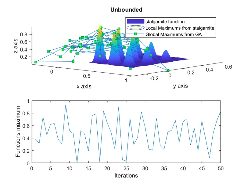
Study 1: Unbounded, we take the inputs as only the stalagmite function & number of the design variables. We measure the time taken for the function to run. We overlap the surface plot of the stalagmite function with the maxima determined the GA at each iteration.
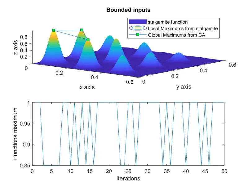
Study 2: Bounded, we take the inputs of lower & upper bounds (to restrict the output of the genetic algorithms) in addition to the stalagmite function & number of design variables. We overlap the surface plot of the stalagmite function with the maxima determined the GA at each iteration.
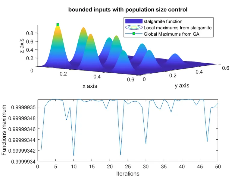
Study 3: Bounded with adjusting the population size: we take the population size (to increase the population size to converge the results quickly) as input in addition to the stalagmite function, number of design variables, lower bound, upper bound. We overlap the surface plot of the stalagmite function with the maxima determined the GA at each iteration.

MATLAB CODE:

clear all
close all
clc

%initial assumption for the x & y regions for which the stalgamite function
%is prepared
x=linspace(0,0.6,150);
y=linspace(0,0.6,150);
[xx yy]=meshgrid(x,y);
%Stalgamit function is run to get the height of the peaks for each
%posistion of the x & y
for i = 1:length(xx)
    for j= 1:length(yy)
        input_1=xx(i,j);
        input_2=yy(i,j);
        input_vectors=[input_1,input_2];
        [f(i,j)]=stalgamite(input_vectors);
        end
end
%initial assumption for the number of iterations the GA to be run is fixed
%as 50
num_cases=50

%Study 1:Unbounded 
tic
for i = 1:num_cases
    [inputs,f_val(i)] = ga(@stalgamite,2);
    x_opt(i)=inputs(1);
    y_opt(i)=inputs(2);
end
study1_time=toc
%plotting the graph to understand the performance of the ga function in
%locating the global maxima
figure(1)
subplot(2,1,1)
hold on
surfc(xx,yy,-f)
xlabel('x axis')
ylabel('y axis')
zlabel('z axis')
shading interp
plot3(x_opt,y_opt,-f_val,'Marker','square','MarkerSize',5,'MarkerFaceColor','g')
legend('stalgamite function','Local Maximums from stalgamite','Global Maximums from GA')
title('Unbounded')
%sub plot to understand the global maximum calculated by the GA algorithm
subplot(2,1,2)
plot(-f_val)
xlabel('Iterations')
ylabel('Functions maximum')

%Study 2:Adding lower & upper bounds for choosing the x & y value

tic
for i = 1:num_cases
    [inputs,f_val(i)] = ga(@stalgamite,2,[],[],[],[],[0,0],[0.6,0.6]);
    x_opt(i)=inputs(1);
    y_opt(i)=inputs(2);
end
study2_time=toc
%plotting the graph to understand the performance of the ga function in
%locating the global maxima
figure(2)
subplot(2,1,1)
hold on
surfc(xx,yy,-f)
xlabel('x axis')
ylabel('y axis')
zlabel('z axis')
shading interp
plot3(x_opt,y_opt,-f_val,'Marker','square','MarkerSize',5,'MarkerFaceColor','g')
legend('stalgamite function','Local Maximums from stalgamite','Global Maximums from GA')
title('Bounded inputs')
%sub plot to understand the global maximum calculated by the GA algorithm
subplot(2,1,2)
plot(-f_val)
xlabel('Iterations')
ylabel('Functions maximum')

%Study 3:adjusting population size with options
options=optimoptions('ga');
options=optimoptions(options,'PopulationSize',300);


tic
for i = 1:num_cases
    [inputs,f_val(i),exitflag] = ga(@stalgamite,2,[],[],[],[],[0,0],[0.6,0.6],[],options);
    x_opt(i)=inputs(1);
    y_opt(i)=inputs(2);
end
study3_time=toc
%plotting the graph to understand the performance of the ga function in
%locating the global maxima
figure(3)
subplot(2,1,1)
hold on
surfc(xx,yy,-f)
xlabel('x axis')
ylabel('y axis')
zlabel('z axis')
shading interp
plot3(x_opt,y_opt,-f_val,'Marker','square','MarkerSize',5,'MarkerFaceColor','g')
legend('stalgamite function','Local maximums from stalgamite','Global Maximums from GA')
title('bounded inputs with population size control')
%sub plot to understand the global maximum calculated by the GA algorithm
subplot(2,1,2)
plot(-f_val)
xlabel('Iterations')
ylabel('Functions maximum')

RESULTS:

Study 1:

Observation: We are not able to achieve the maxima in this study which is evident from the first plot & a time taken is 2.7 secs

From the plot 1: We can find that the determined maxima outside of the bounds of the stalagmite function. We find the Global maximums from GA in the negative of x & y where the stalagmite function is not available in this example.

From the plot 2: We can see that the maximums from GA is ranging from 0 to 1 in the 50 iterations

Study 2:

Observation: We are able to reduce the number of maxima compared to the previous study but still the global maxima has not been identified & time taken is 3.35 secs

From the plot 1: We can see that Global maximums from GA are narrowed the global maximum to the biggest three peaks of the stalagmite function

From the plot 2: We can see that the maximums from GA is now ranging only from 0.85 to 1 & also majority of the iterations have maximum as 1.

Study 3:

Observation :We are able to determine the global maxima after increasing the population size to 300 & time taken is 9.57 secs. hence due to longer duration with the increase in population has to be done with caution.

From the plot 1: We can see that the global maximum from GA is actually the global maximum of the stalagmite function pictorically.

From the plot 2: We can see that the variations of the global maximum across iterations is on the 6th decimal which is a good level of accuracy.