Week 5 - Curve fitting
CURVE FITTING
OBJECTIVE:
To fit a linear & cubic polynomial for the given Cp data & compare the two to understand which equation provides a better fit. To determine the goodness of fit for the above equations & explain the next actions to reach the best fit for the given Cp data.
PROBLEM STATEMENT:
Curve fitting is the one of the processes to determine & understand the relationship between a system of variables. Based on the relationship we will be able to determine the y value with required x value which could be interpolating or extrapolating the existing data.
To understand the relationship between the variables, we need to know the goodness of fit i.e., how much accurately y value can be predicted by the fitting equation. We have few methods to calculate the goodness of fit like R-square, RMSE etc.
- R square: This value ranges from 0 to 1 which shows the connection between the dependant variable & independent variable. Value close to 1 shows the stronger connection between the two variables but this does not inform about causality.
- RMSE (Root mean square of error): Square root of the variance of the residuals or errors. It indicates the absolute fit of the model to the data–how close the observed data points are to the model’s predicted values. It has the useful property of being in the same units as the response variable. Lower values of RMSE indicate better fit.
In this project we have been requested to provide the fitting equation in the form of linear & cubic polynomial. Additionally, to reach the best fit for the given Cp data we have studied with the four, five, six-degree polynomial and logarithmic equation.
THEORITICAL QUESTIONS:
- Popt holds the array of optimal parameters or coefficients of the function used for fitting the curve so that the sum of squared error of f(x)-y data is a minimum value. Pcov holds the 2d array of estimated covariance of the parameters, whose diagonal provides the variance of the parameter estimate.
- np.array(temperature) converts the temperature list to NumPy array which allows to access all values inside temperature list for computing the Calculated Cp with optimised parameters.
- * in *popt means to access all parameters in the popt array to the function to calculate new cp values based on these parameters.
SOLUTION PROCEDURE:
- The functions for reading the file are created where each line is splitted using split command & comma as the delimiter. The temperature & Cp data are stored into their respective lists.
- The functions are created for all fitting functions (linear, cubic, four-degree, five-degree, six-degree, logarithmic equation)
- Curve fit function takes inputs as fitting function, temp data, Cp data and gives output as an array of optimised parameters & an 2D array of covariance of parameters.
- Cp data is calculated with optimised parameters in the fitting function
- Function is created to calculate the goodness of fit in which
- Inputs: The Actual Cp & Calculated Cp with optimal parameters & mean for actual Cp
- Calculation: Error is calculated by the difference between the actual Cp & Calculated Cp & Difference between the Calculated Cp with Mean for actual Cp is calculated. Based on these two estimations, we determine the R square & RMSE.
- Outputs: R square, RMSE & Error
- Plot is created with Actual Cp & Calculated Cp for all equations
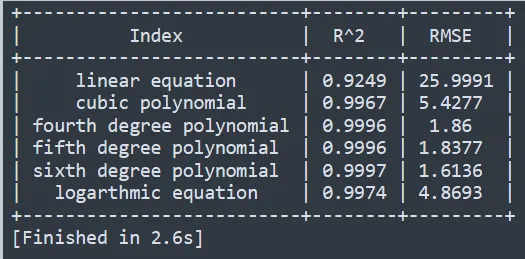
- Tabulating the R square & RMSE for all equations for easy comparison.
CODE REFERENCE:
import numpy as np
import matplotlib.pyplot as plt
from scipy.optimize import curve_fit
from tabulate import tabulate
#Function list for curve fitting
def log_func(t,a,b):
	return a*np.log(t)+b

def cubic_func(t,a,b,c,d):
	return a*pow(t,3)+b*pow(t,2)+c*t+d

def linear_func(t,a,b):
	return a*t+b
def four_func(t,a,b,c,d,e):
	return a*pow(t,4)+b*pow(t,3)+c*pow(t,2)+d*t+e

def five_func(t,a,b,c,d,e,f):
	return a*pow(t,5)+b*pow(t,4)+c*pow(t,3)+d*pow(t,2)+e*t+f

def six_func(t,a,b,c,d,e,f,g):
	return a*pow(t,6)+b*pow(t,5)+c*pow(t,4)+d*pow(t,3)+e*pow(t,2)+f*t+g

#Function for reading files
def read_file():
	temperature=[]
	Cp=[]
	f=open('data for temp & Cp','r')
	for line in f:
		values=line.split(',')
		temperature.append(float(values[0]))
		Cp.append(float(values[1]))

	return [temperature,Cp]

#Function for estimating the goodness of fit with Rsq & RMSE
def goodness_fit(y,fit_y,D_mean):
	Error_sq=[]
	Error=[]
	SSR=[]
	for i in range(0,len(cp)):
		error_i=y[i]-fit_y[i]
		ssr_i=fit_y[i]-D_mean
		Error.append(error_i)
		Error_sq.append(pow(error_i,2))
		SSR.append(pow(ssr_i,2))
	SST=sum(Error_sq)+sum(SSR)
	R_sq=sum(SSR)/SST
	RMSE=np.sqrt((sum(Error_sq))/len(cp))
	return(R_sq,RMSE,Error)


temp , cp= read_file()
Data_mean=np.mean(cp)

#Paraemeters for logarthmic function
popt_log,pcov_log=curve_fit(log_func,temp,cp)
fit_cp_log=log_func(np.array(temp),*popt_log)

#Error calculation by R2 method
Error_log=[]
R_sq_log,RMSE_log,Error_log=goodness_fit(cp,fit_cp_log,Data_mean)


#Plotting the actual data vs curve_fit
plt.figure()
plt.plot(temp,cp,color="blue",linewidth=3)
plt.plot(temp,fit_cp_log,color="red",linewidth=2)
plt.text(1300,1300,"$R^2=%f$"%R_sq_log,fontsize=8,bbox=dict(facecolor="grey",alpha=0.5))
plt.text(1300,1265,"$RMSE=%f$"%RMSE_log,fontsize=8,bbox=dict(facecolor="grey",alpha=0.5))
plt.legend(['Actual data','Curve fit'])
plt.xlabel('Temperature in K')
plt.ylabel('Cp')
plt.title("Actual data vs Curve fit with logarthmic equation")
plt.savefig("Actual data vs curve_fit with logarthmic equation")
#Plotting Error vs temp
plt.figure()
plt.scatter(temp,Error_log,marker='o')
plt.xlabel('Temperature in K')
plt.ylabel('Error (Y(i)- f(x(i))')
plt.title("Error vs Temp for logarthmic equation")
plt.savefig("Error of logarthmic equation with actual data vs Temp")


#Linear function
popt_linear,pcov_linear=curve_fit(linear_func,temp,cp)
fit_cp_linear=linear_func(np.array(temp),*popt_linear)

#Error calculation by R2 method
Error_linear=[]
R_sq_linear,RMSE_linear,Error_linear=goodness_fit(cp,fit_cp_linear,Data_mean)


#Plotting the actual data vs curve_fit
plt.figure()
plt.plot(temp,cp,color="blue",linewidth=3)
plt.plot(temp,fit_cp_linear,color="red",linewidth=2)
plt.text(1300,1300,"$R^2=%f$"%R_sq_linear,fontsize=8,bbox=dict(facecolor="grey",alpha=0.5))
plt.text(1300,1265,"$RMSE=%f$"%RMSE_linear,fontsize=8,bbox=dict(facecolor="grey",alpha=0.5))
plt.legend(['Actual data','Curve fit'])
plt.xlabel('Temperature in K')
plt.ylabel('Cp')
plt.title("Actual data vs Curve fit with linear polynomial")
plt.savefig("Actual data vs Curve fit with linear polynomial")
#Plotting Error vs temp
plt.figure()
plt.scatter(temp,Error_linear,marker='o')
plt.xlabel('Temperature in K')
plt.ylabel('Error (Y(i)- f(x(i))')
plt.title("Error vs Temp for linear polynomial")
plt.savefig("Error of linear polynominal with actual data vs Temp")


#cubic function
popt_cubic,pcov_cubic=curve_fit(cubic_func,temp,cp)
fit_cp_cubic=cubic_func(np.array(temp),*popt_cubic)

#Error calculation by R2 method
Error_cubic=[]
R_sq_cubic,RMSE_cubic,Error_cubic=goodness_fit(cp,fit_cp_cubic,Data_mean)


#Plotting the actual data vs curve_fit
plt.figure()
plt.plot(temp,cp,color="blue",linewidth=3)
plt.plot(temp,fit_cp_cubic,color="red",linewidth=2)
plt.text(1300,1300,"$R^2=%f$"%R_sq_cubic,fontsize=8,bbox=dict(facecolor="grey",alpha=0.5))
plt.text(1300,1265,"$RMSE=%f$"%RMSE_cubic,fontsize=8,bbox=dict(facecolor="grey",alpha=0.5))
plt.legend(['Actual data','Curve fit'])
plt.xlabel('Temperature in K')
plt.ylabel('Cp')
plt.title("Actual data vs Curve fit with cubic polynomial")
plt.savefig("Actual data vs curve_fit with cubic polynomial")
#Plotting Error vs temp
plt.figure()
plt.scatter(temp,Error_cubic,marker='o')
plt.xlabel('Temperature in K')
plt.ylabel('Error (Y(i)- f(x(i))')
plt.title("Error vs Temp for cubic polynomial")
plt.savefig("Error of cubic polynominal with actual data vs Temp")
#four function
popt_four,pcov_four=curve_fit(four_func,temp,cp)
fit_cp_four=four_func(np.array(temp),*popt_four)

#Error calculation by R2 method
Error_four=[]
R_sq_four,RMSE_four,Error_four=goodness_fit(cp,fit_cp_four,Data_mean)


#Plotting the actual data vs curve_fit
plt.figure()
plt.plot(temp,cp,color="blue",linewidth=3)
plt.plot(temp,fit_cp_four,color="red",linewidth=2)
plt.text(1300,1300,"$R^2=%f$"%R_sq_four,fontsize=8,bbox=dict(facecolor="grey",alpha=0.5))
plt.text(1300,1265,"$RMSE=%f$"%RMSE_four,fontsize=8,bbox=dict(facecolor="grey",alpha=0.5))
plt.legend(['Actual data','Curve fit'])
plt.xlabel('Temperature in K')
plt.ylabel('Cp')
plt.title("Actual data vs Curve fit with four degree equation")
plt.savefig("Actual data vs curve_fit with four degree equation")
#Plotting Error vs temp
plt.figure()
plt.scatter(temp,Error_four,marker='o')
plt.xlabel('Temperature in K')
plt.ylabel('Error (Y(i)- f(x(i))')
plt.title("Error vs Temp for four degree equation")
plt.savefig("Error of four degree equation with actual data vs Temp")

#five function
popt_five,pcov_five=curve_fit(five_func,temp,cp)
fit_cp_five=five_func(np.array(temp),*popt_five)

#Error calculation by R2 method
Error_five=[]
R_sq_five,RMSE_five,Error_five=goodness_fit(cp,fit_cp_five,Data_mean)


#Plotting the actual data vs curve_fit
plt.figure()
plt.plot(temp,cp,color="blue",linewidth=3)
plt.plot(temp,fit_cp_five,color="red",linewidth=2)
plt.text(1300,1300,"$R^2=%f$"%R_sq_five,fontsize=8,bbox=dict(facecolor="grey",alpha=0.5))
plt.text(1300,1265,"$RMSE=%f$"%RMSE_five,fontsize=8,bbox=dict(facecolor="grey",alpha=0.5))
plt.legend(['Actual data','Curve fit'])
plt.xlabel('Temperature in K')
plt.ylabel('Cp')
plt.title("Actual data vs Curve fit with five degree equation")
plt.savefig("Actual data vs curve_fit with five degree equation")
#Plotting Error vs temp
plt.figure()
plt.scatter(temp,Error_five,marker='o')
plt.xlabel('Temperature in K')
plt.ylabel('Error (Y(i)- f(x(i))')
plt.title("Error vs Temp for five degree equation")
plt.savefig("Error of five degree equation with actual data vs Temp")


#six function
popt_six,pcov_six=curve_fit(six_func,temp,cp)
fit_cp_six=six_func(np.array(temp),*popt_six)

#Error calculation by R2 method
Error_six=[]
R_sq_six,RMSE_six,Error_six=goodness_fit(cp,fit_cp_six,Data_mean)


#Plotting the actual data vs curve_fit
plt.figure()
plt.plot(temp,cp,color="blue",linewidth=3)
plt.plot(temp,fit_cp_six,color="red",linewidth=2)
plt.text(1300,1300,"$R^2=%f$"%R_sq_six,fontsize=8,bbox=dict(facecolor="grey",alpha=0.5))
plt.text(1300,1265,"$RMSE=%f$"%RMSE_six,fontsize=8,bbox=dict(facecolor="grey",alpha=0.5))
plt.legend(['Actual data','Curve fit'])
plt.xlabel('Temperature in K')
plt.ylabel('Cp')
plt.title("Actual data vs Curve fit with six degree equation")
plt.savefig("Actual data vs curve_fit with six degree equation")
#Plotting Error vs temp
plt.figure()
plt.scatter(temp,Error_six,marker='o')
plt.xlabel('Temperature in K')
plt.ylabel('Error (Y(i)- f(x(i))')
plt.title("Error vs Temp for six degree equation")
plt.savefig("Error of six degree equation with actual data vs Temp")

#Tabulating results
Index=("linear equation","cubic polynomial","fourth degree polynomial","fifth degree polynomial","sixth degree polynomial","logarthmic equation")
R_sq=(round(R_sq_linear,4),round(R_sq_cubic,4),round(R_sq_four,4),round(R_sq_five,4),round(R_sq_six,4),round(R_sq_log,4))
RMSE=(round(RMSE_linear,4),round(RMSE_cubic,4),round(RMSE_four,4),round(RMSE_five,4),round(RMSE_six,4),round(RMSE_log,4))

Table=zip(Index,R_sq,RMSE)
Headers=("Index","R^2","RMSE")
print(tabulate(Table,headers=Headers,tablefmt="pretty"))
RESULTS:
Key points arrived from the below data
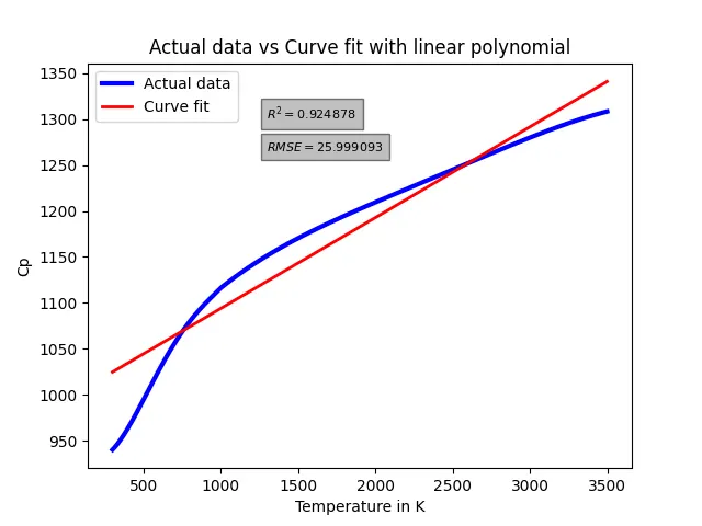
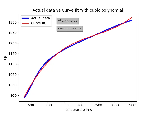
- Based on comparison between the linear & cubic polynomial, we conclude the cubic polynomial is a better fit to the input data.
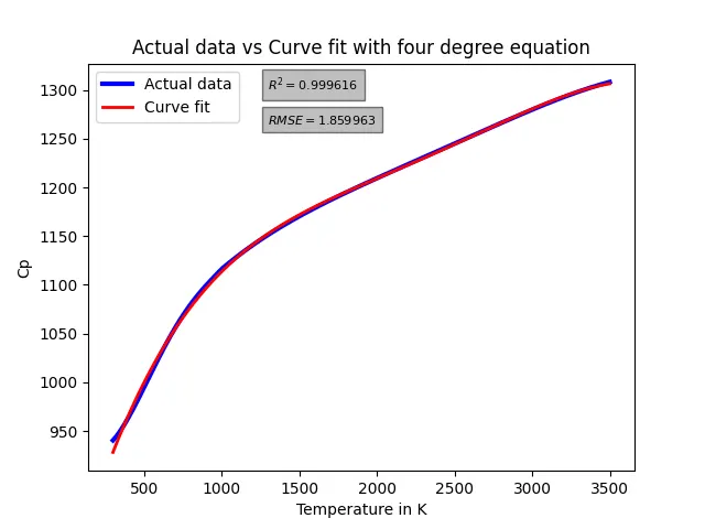
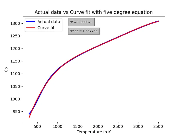
- We are able to achieve the better fit by increasing the degree of the polynomial as we found in the below examples
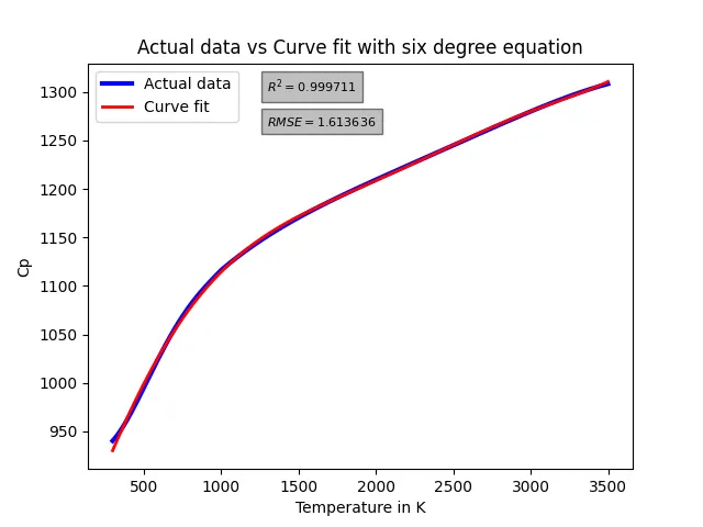
- From the table of results, we are able to conclude the sixth-degree polynomial is the best fit among all equations used in this program since it has
- R square value of 0.9997 which is close to 1 (max limit of R square)
- RMSE of 1.6136 (lowest error of all equations) confirming this is the best fit
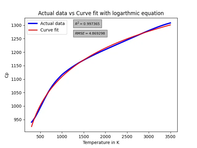
- For comparison we have studied with logarithmic equation, which is slightly better than cubic but lesser than the fourth-degree polynomial
Actual Cp with Calculated Cp for linear equation
Actual Cp with Calculated Cp for cubic polynomial equation
Actual Cp with Calculated Cp for fourth degree polynomial equation
Actual Cp with Calculated Cp for fifth degree polynomial equation
Actual Cp with Calculated Cp for sixth degree polynomial equation
Actual Cp with Calculated Cp for logarithmic equation
Tabulate the results of R square & RMSE for all fitting equations
DISCUSSION
Based on the above project, we are able to understand the curve fitting for the given input data and also determining the goodness of fit for the fitting equation by comparing the error in dependent variable calculation.
To better understand the application in practical situation, we should work on the real-life estimations whose study could be an interesting next scope. When working on the next scope we should also focus on making the code more dynamic.
REFERENCE:
- https://docs.scipy.org/doc/scipy-0.16.1/reference/generated/scipy.optimize.curve_fit.html
- https://towardsdatascience.com/basic-curve-fitting-of-scientific-data-with-python-9592244a2509