Week 3 - Solving second order ODEs

SIMULATION OF SIMPLE PENDULUM BY SOLVING SECONG ORDER ODE’S

OBJECTIVE:

To understand the relationship between displacement & velocity of the pendulum with time variable by solving the second order differential equations and also show the simulation of the simple pendulum in python.

PROBLEM STATEMENT:

A pendulum moves in simple harmonic motion generally with smaller displacements.When there is no external influence of the pendulum the free body diagram of the pendulum will appear like shown in below image

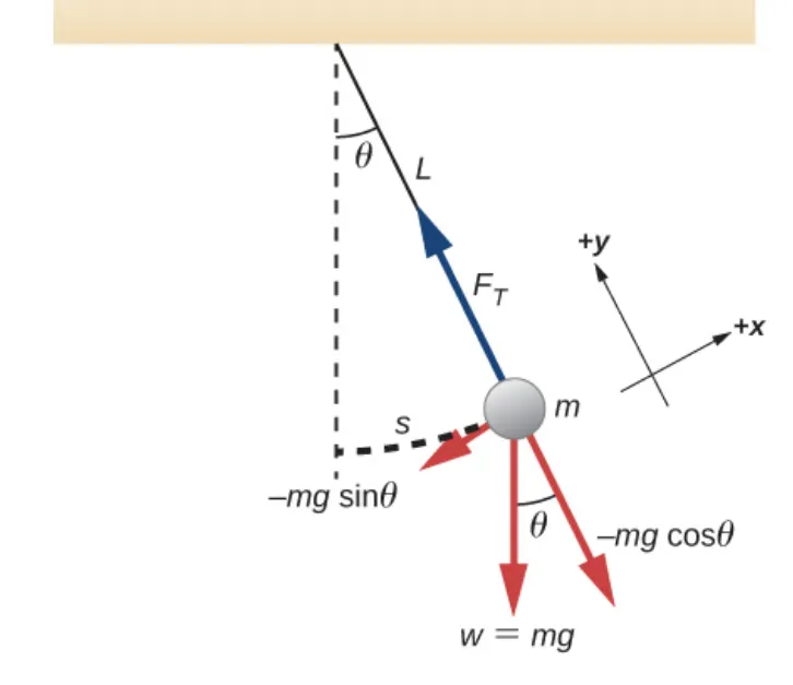
Here the gravitational effect on the mass can be resolved into two radial & tangential forces. The radial force is directly opposing the tension of the string which cancels it. So, the tangential force is acting on the mass which is opposed by the damping effect which is due to the friction at the fixation & air resistance.

The motion of the pendulum can be determined by the below equation which explains the displacement & velocity of the pendulum.

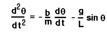
Where,

θ is the angle formed by the string with fixation

So the first derivative is the angular displacement & second derivative is the velocity

b is the damping coefficient

L is the length of the string

m is the mass at the end of string

In this project we will determine relationship between the displacement & velocity with respect to time. Then we determine the position of the pendulum at various time frames & create a animation file for showing the motions of the simple pendulum

SOLUTION PROCEDURE:

We will be able to the solve second order ODE with the help of odeint function in the scipy library. Firstly we have to breakdown the second ODE to two first ODE to easily solve for the desired outputs

We can breakdown it to two first order ODE like below with the assumption u = θ,

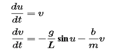
Hence by solving two first order ODE we will be able to determine the displacement & velocity of pendulum.

We have the below code structured in the following steps

• The following inputs are assumed for this calculation
  1. Length of the string
  2. Mass of the string (negligible so zero)
  3. Mass at the end of spring
  4. Damping coefficient
  5. Initial condition (angle & velocity of the pendulum)
• Function definition with the two first order ODE inside the function block & returning the displacement & velocity
• Solving for the displacement & velocity with the help of odeint & defined function for the number of time intervals required.
• Creating the multiple images of the pendulum with the help of the angular displacement obtained in the previous step.
• Combining the multiple images into the gif & then combining the gif file to mp4

CODE REFERENCE:

import math
import matplotlib.pyplot as plt
import numpy as np
from scipy.integrate import odeint
from PIL import Image
import glob
import moviepy.editor as mp

"""
1st section: Creating relation between displacement & velocity with respect to time
Inputs
b : damping coefficient 
m : mass in kg
g : acceleration due to gravity in m/s2 : 9.81 ( constant)
L : length of the pendulum (m)
t : time array 
Mass of the string is assumed as zero
theta : 0 is for displacement & 1 is for velocity
so output will have 1st column is for displacement, 2nd column is for velocity with t number of rows
"""



b= 0.05
m = 1
g = 9.8
L = 1
t=np.linspace(0,20,150)


# Initial condition is pushing the pendulum with 3 m/s2 velocity from zero deg 
theta_0=[0,3]

# function definition
def model(theta,t,b,m,L,g):
	theta1 = theta[0]
	theta2 = theta[1]

	dtheta_1=theta2
	dtheta_2=((-b/m)*theta2)-((g/L)*math.sin(theta1))
	dtheta_dt=[dtheta_1,dtheta_2]
	return dtheta_dt



# Solve ODE
theta = odeint(model,theta_0,t,args = (b,m,L,g))
# PLOTTING
plt.figure()
plt.plot(t,theta[:,0],'b--',label=r'$\frac{d\theta_1}{dt}=\theta_2$')
plt.plot(t,theta[:,1],'r--',label=r'$\frac{d\theta_2}{dt}=-\frac{b}{m}\theta_2-\frac{g}{L}sin\theta_1$')
plt.xlabel("Time")
plt.ylabel("Displacement in m & velocoity in m/s2")
plt.title("Displacement & velocity vs time")
plt.legend(loc='best')
plt.savefig("Displacement & Velocity vs time.jpg")

#2nd section : Pendulum animation section
#part A: Creating multiple images

#string centre
x0=0
y0=0
#countervariable
ct=1
for i in theta[:,0]:
	#end co-ordinates of the bob
	x1=L*math.sin(i)
	y1=-L*math.cos(i)
	filename=" output %05d.png" %ct
	plt.figure()
	#plotting the string
	plt.plot([x0,x1],[y0,y1])
	plt.plot(x1,y1,marker='o',markerfacecolor='red',markersize=12)
	#plotting the fixation by a line
	plt.plot([-0.25,0.25],[0,0],color='black',linewidth=4)
	axis_invisble=plt.gca()
	axis_invisble.axes.xaxis.set_visible(False)
	axis_invisble.axes.yaxis.set_visible(False)
	plt.xlim([-1.5,1.5])
	plt.ylim([-1.5,0.5])
	plt.savefig(filename)
	ct=ct+1

#Part B : Converting png to gif
Frames=[]
png_path="D:/python/Challenges/Week 3_second order ODE's/*.png"
imgs=glob.glob(png_path)
for i in imgs:
	new_frame = Image.open(i)
	Frames.append(new_frame)

Frames[0].save('png_to_gif.gif', format='GIF',append_images=Frames[1:],save_all=True,duration=100, loop=0)


#Part C: gif to mp4 creation
#Gif file is read by the videofileclip 
Video_clip=mp.VideoFileClip("png_to_gif.gif")
#Write_videofile for creating a video file with the above gif
#Video is created with fps 24 as default
Video_clip.write_videofile("Simple pendulum with damper.mp4")

ERROR & SOLUTIONS:

Error 1: Output image was opened, so program was not able to rewrite the file with new image, it got rectified once it was rerun after closure of the image.

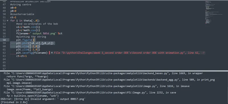
Error 2: Pendulum image was upside down

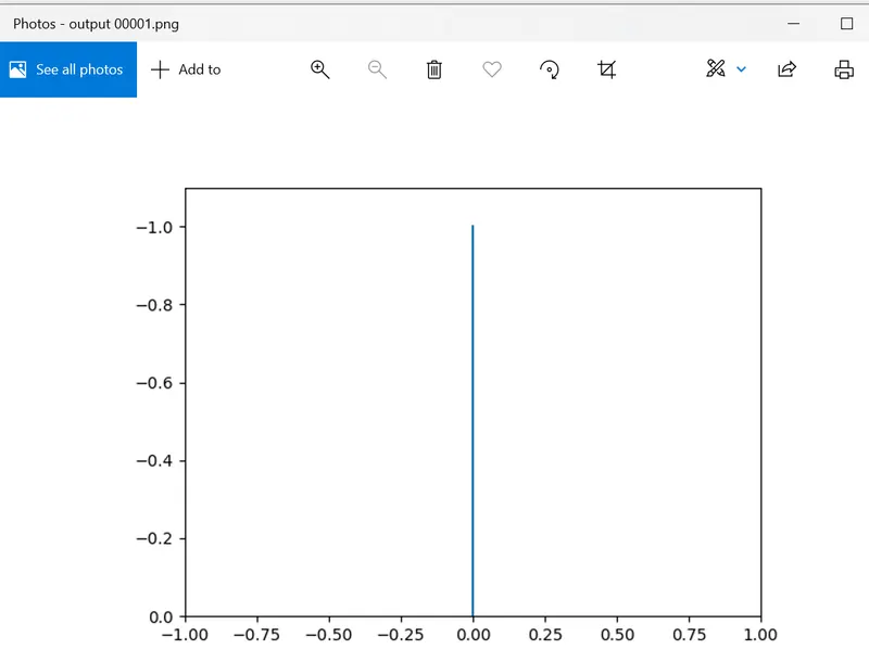
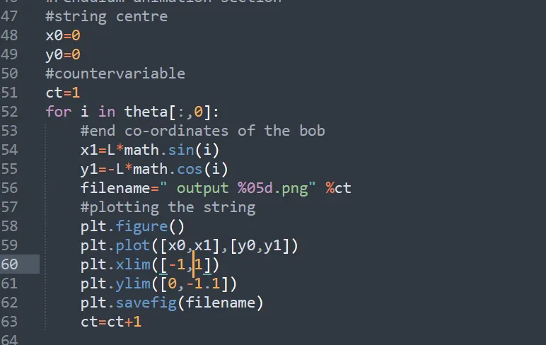
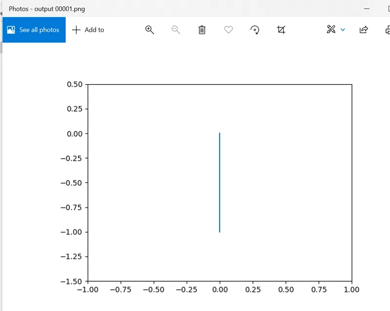
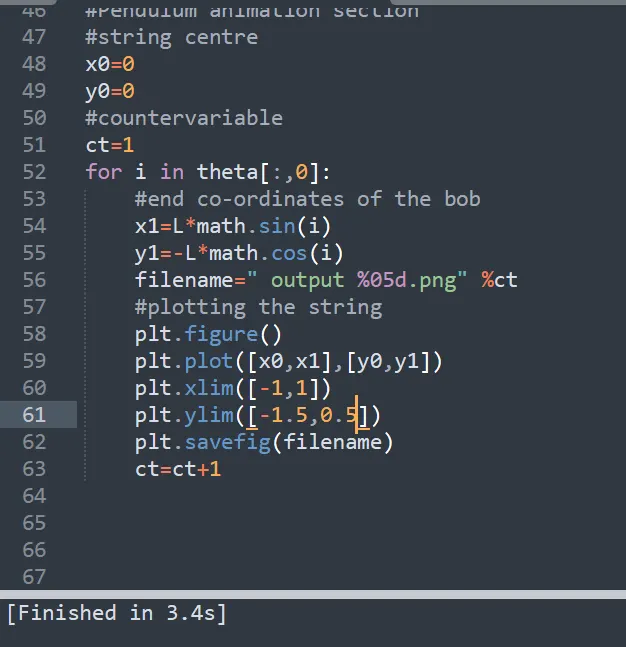
Once the axis limit value was changed from (0,-1.1) to (-1.5,0.5), the solution was as desired

Hence the learning here was to define the lower limit first followed by the upper limit

RESULTS

We have the plot which describes the displacement & velocity with respect to time

Animation file link for the motion of the pendulum

https://youtu.be/PEe4cyuo2pg

DISCUSSION

Based on the above project, we are able to understand the relationship between the displacement & velocity with the respect to the time period. We have calculated the motion of the simple pendulum with the assumption of the mass of the string is negligible.

To better understand the situation, we should study the forces acting on the pendulum at various stages of its motion. Analysing these forces with the inclusion remaining influencing parameters could be an interesting next scope.

REFERENCE:

• https://services.math.duke.edu/education/postcalc/predprey/appendix.html