Week 2 Air standard Cycle

SIMULATION OF AIR STANDARD OTTO CYCLE

OBJECTIVE:

To simulate the PV plot of the Ideal Otto cycle with the determination of the state variables using python & the efficiency for the Ideal cycle.

PROBLEM STATEMENT:

Otto Cycle is a one of the commonly used methods to generate energy from fuels like gasoline. Otto cycle converts the chemical energy of the fuel into thermal energy which is then expanded to produce kinetic energy. The Otto cycle is generally used by the automobile industry for transportation. Otto cycle generally consists of the following stages

• Intake stroke (5->1): Intake valve is opened & Air & Fuel mixture enter into the engine cylinder
• Isentropic compression stroke (1-> 2): Piston moves from Bottom dead centre to the Top dead centre. Compression of the mixture which increases the pressure & temperature & decreases the volume.
• Isochoric heat addition (2-> 3): Spark ignition occurs for a short duration which results in increase of the pressure & temperature at constant volume.
• Isentropic expansion stroke (3-> 4): Piston is pushed down from top dead centre to the bottom centre by the force of controlled combustion. During expansion the pressure & temperature decreases with increase in volume
• Isochoric heat rejection (4-> 1): Heat is rejected by the engine in constant volume with the decrease in the pressure & temperature
• Exhaust stroke (1-> 5): Exhaust gases are pushed outside by opening of the exhaust valve.

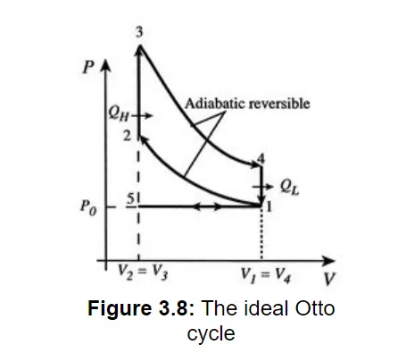
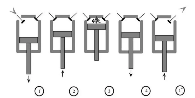
PV diagram is one of the graphs required to understand the Otto cycle which shows the pressure and volume of the gas during various stages. In this project we will determine temperature, pressure & volume at various stages of the otto cycle with the specified inputs & also compute the efficiency of the engine.

SOLUTION PROCEDURE:

Governing equations for Otto cycle:

• Volume as function of the crank angle

• Pressure & Volume for isentropic process : P * (V^gamma) = Constant

where gamma is gas constant

• Pressure, Volume & temperature for the Ideal gas : P * V = n* R * T

In this scenario, where there is no external interaction, we can consider (P * V)/ T = constant

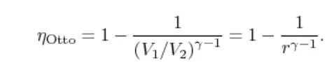
• Efficiency of Otto cycle:

• Swept volume = (pi()/4)* (diameter of the bore ^ 2) * (stroke )

• Clearance volume = Swept volume/(compression ratio – 1)

We have the below code structured in the following steps

• The following inputs are assumed for this calculation
  1. Geometric dimensions of the cylinder
  2. Pressure & temperature of the initial stage & gas constant
  3. Compression ratio of the engine
• Computation of the swept volume, Clearance volume & Initial Volume.
• Determination of the pressure & temperature with ideal gas law & isentropic equations.
• Determination of the pressure & Volume during compression & expansion with the equation which provides the volume of gas at various angles of the crank.
• Calculation of the efficiency with compression ratio
• Plotting the PV plot with ideal otto cycle with various state points
• Additionally, we have plotted the Change in efficiency with the various compression ratio.

CODE REFERENCE:

import math
import matplotlib.pyplot as plt
import numpy as np

#Function to calculate the Volume & pressure values with crank angle for the expansion & compressure
def Engine_kinematics(bore,stroke,con_rod,cr,start_angle,end_angle,n):
	# geometric dimensions of engine
	a= stroke/2
	R= con_rod/a

	# Volume parameters
	V_s=(math.pi/4)*pow(bore,2)*stroke
	V_c=V_s/(cr-1)

	# Crank angle
	V=[]
	crank_angle =np.linspace(start_angle,end_angle,n)
	for i in range(0,n):
		theta = math.radians(crank_angle[i])
		

		# Volume trace calculation
		term1= 0.5*(cr-1)
		term2= (R+1-math.cos(theta))
		term3= pow(R,2)-pow(math.sin(theta),2)
		term4= pow(term3,0.5)
		V.append((1+term1*(term2-term4))*V_c)

	return(V)




#input variables
p0= 101325
p1=p0
t1= 500
gamma =1.4
t3= 2500
# geometric dimensions of engine
bore = 0.1
stroke = 0.1
con_rod = 0.156
cr= 8
#number of steps required to calculate in between stages for compression & expansion
n=50

# Volume computation
V_s	= (math.pi/4)*pow(bore,2)*stroke
V_c = V_s/(cr-1)
V0=V_c
V1 = V_s+V_c

# state point 2
V2= V_c
# PV^gamma is constant
p2= (p1*pow(V1,gamma))/(pow(V2,gamma))
#PV/T is constant for all state variable
rhs = ((p1*V1)/t1)
t2 = (p2*V2)/rhs 

V_compression= Engine_kinematics(bore,stroke,con_rod,cr,180,0,n)
P_compression=[]
constant=p1*pow(V1,gamma)
for v in V_compression:
	P_compression.append(constant/pow(v,gamma))

#state point 3
V3=V2
#PV/T is constant for all state variable
p3=(rhs*t3)/V3

V_expansion= Engine_kinematics(bore,stroke,con_rod,cr,0,180,n)
P_expansion=[]
constant=p3*pow(V3,gamma)
for v in V_expansion:
	P_expansion.append(constant/pow(v,gamma))

# state point 4
V4= V1
# PV^gamma is constant
p4= (p3*pow(V3,gamma))/(pow(V4,gamma))
#PV/T is constant for all state variable
rhs = ((p3*V3)/t3)
t4 = rhs/(p3*V3)

#Efficiency of the Otto cycle
sub_term = pow(cr,(gamma-1))
Efficiency = round((1 - (1/sub_term))*100,2)
print("Efficiency of the Otto engine is", Efficiency, "%")

#Plotting of the Ideal Otto cycle
plt.plot([V0,V1],[p0,p1],label="Intake & Exhaust stroke")
plt.plot(V_compression,P_compression,label="Isochroric heat addition process")
plt.plot([V2,V3],[p2,p3],label="Isentropic compression process")
plt.plot(V_expansion,P_expansion,label="Isochroric heat rejection process")
plt.plot([V4,V1],[p4,p1],label="Isentropic expansion process")
plt.title("PV GRAPH FOR IDEAL OTTO CYCLE")
plt.xlabel("Volume in m3")
plt.ylabel("pressure in pascal")
plt.legend()
plt.show()


# To compute efficiency vs compression ratio
#Compression ratio
Compression_ratio = np.linspace(1,16,32)
#Empty array for Efficiency
Eff =[]
#Calculating efficiency for each compression ratio
for i in Compression_ratio:
	sub = pow(i,(gamma-1))
	Eff.append(round((1 - (1/sub))*100,2))
#Plotting the graph for efficiency vs compression ratio
plt.plot(Compression_ratio,Eff)
plt.title("Efficiency Vs Compression ratio")
plt.xlabel("Compression ratio")
plt.ylabel("Efficiency")
plt.show()

RESULTS

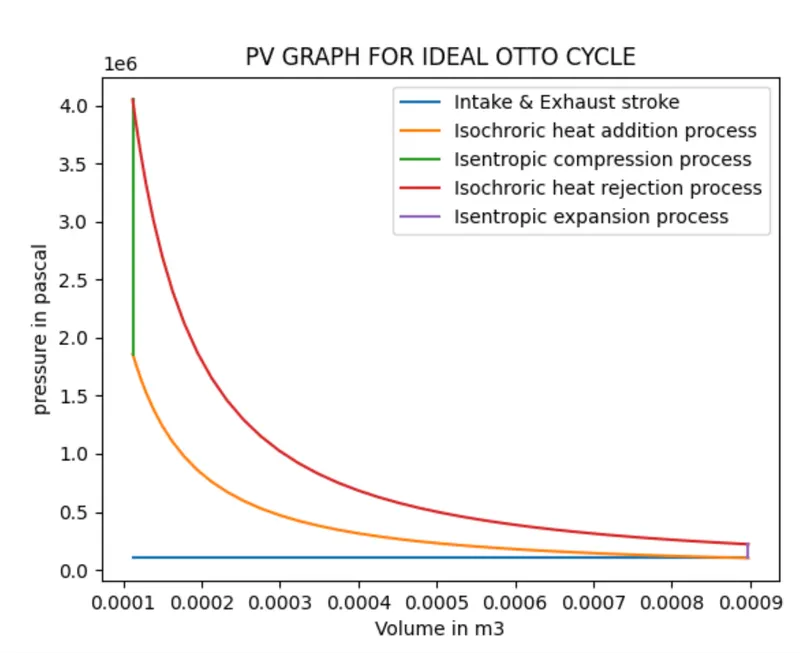
We have the desired PV plot for the ideal Otto cycle attached below

Efficiency of the otto cycle is shown in the output

Efficiency vs compression ratio plot is mentioned below

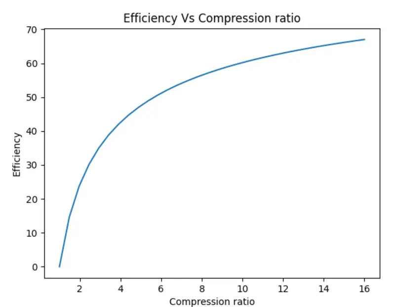
Based on PV plot, we understand the variation of pressure & volume at various stages of the otto cycle. Based on the efficiency vs compression ratio, we understand the efficiency increases with the increase in compression ratio up to certain limit drastically but after that it is increasing very slowly.

DISCUSSION

Based on the above project, we are able to understand the pressure, volume & temperature for the otto cycle at various stages. We have calculated with the help of ideal gas law & isentropic equation condition for the ideal scenario.

In a real-life situation where there are other influencing parameters where the ideal gas law & isentropic equation are not directly applicable. Analysing some of the factors to make the project closer to the practical scenario could be an interesting next scope.

REFERENCE: MIT Course content https://web.mit.edu/16.unified/www/FALL/thermodynamics/notes/node26.html