Week 4.1 - Genetic Algorithm

AIM: To find the global maxima of a function by using genetic algorithm in MATLAB.

OBJECTIVE:

• To study about Genetic Algorithm and Stalagmite function.
• To write code in matlab to optimise the stalagmite function and find the Global maxima of the function.
• To plot the graphs based on the study done on Genetic Algorithm.

THEORY:

Genetic algortihm:

Genetic algorithm solves smooth or nonsmooth optimization problems with any types of constraints, including integer constraints. It is a stochastic, population-based algorithm that searches randomly by mutation and crossover among population members. In a genetic algorithm, a population of candidate solutions (called individuals, creatures, or phenotypes) to an optimization problem is evolved toward better solutions. Each candidate solution has a set of properties which can be mutated and altered; traditionally, solutions are represented in binary as strings of 0s and 1s, but other encodings are also possible.

The genetic algortihm uses three main types of rules at each step to create the next population from the current population.

1. Selection rules selects the individuals, called parents, that contributes to the population in the next generation.
2. Crossover rules combines two parents to form children for the next generation.
3. Mutation rules apply random changes to individual parents to form children.

How does the genetic algorithm works?

1. The algorithm begins by creating a random population.
2. The algorithm then creates a sequence of new populations. At each step, the algorithm uses the individuals in current population to create the next population. The algorithm performs some defined steps to create new population.
   
   (i) Scores each member of the current population by computing its fitness value. The values are called raw fitness scores.
   (ii) Scales the raw fitness scores to convert it into a more usable range of values. These scaled values are called expectation values.
   (iii) Select the members and call the parents based on their expectation values.
   (iv) Individuals having lower fitness values in the current population are to as elite, which further passed to the next population.
   (v) Then the childrens are produced from the parents. it is done by making random changes to the parents,known as mutation or by combining the vector entries of a pair of parents which is called crossover
   
   
3. The algorithm stops when one of the stopping criteria is met.

Genetic algorithm syntax used in the program:

1. x = ga(@func,nvars), where "func" is the function name and "nvars" is the number of variables.

2. x = ga(@func,nvars,A,B,Aeq,Beq)

3. x = ga(@func,nvars,A,B,Aeq,Beq,lb,ub,nonlcon,intcon,options), where
A,B = linear inequality constraints
Aeq,Beq = linear equality constraints
lb = lower bound
ub = upper bound
nonlcon = nonliner constraints
intcon = vector of positive integers
options = optimization options

Stalagmite function:

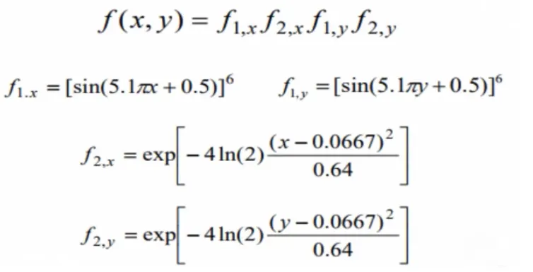
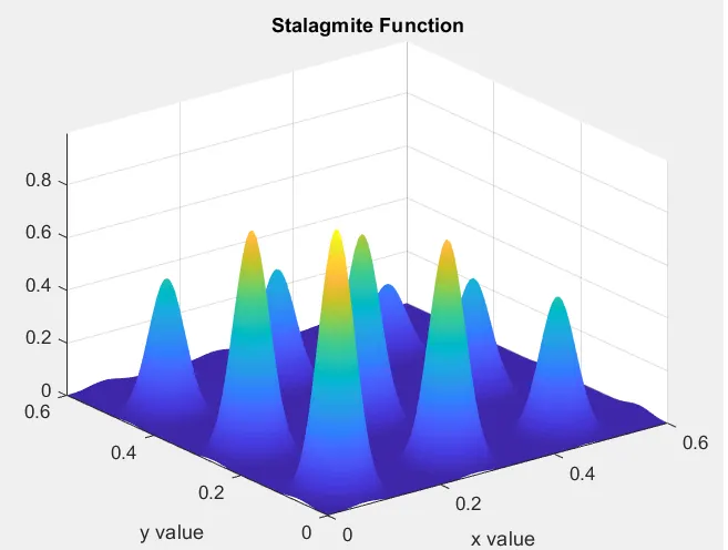
A stalagmite function generally refers to the function with which we are generating values over a stalagmite kind of surface for finding out the local and global maxima and minima of that particular given function.

There are following equations used for the stalagmite function mentioned below:

Function code:

function [f]= stalagmite(input_vector)
a=input_vector(1);
b=input_vector(2);
term1 = (sin((5.1*pi*a)+0.5))^6
term2 = exp(-4*log(2)*((a-0.0667)^2)/0.64); 
term3 = (sin((5.1*pi*b)+0.5))^6
term4 = exp(-4*log(2)*((b-0.0667)^2)/0.64);

[f] = -(term1*term2*term3*term4);

end

Program Code:

clear all 
close all
clc

% Defining search space
x = linspace(0,0.6,150);
y = linspace(0,0.6,150);
%creating a 2D meshg
[xx,yy] = meshgrid(x,y)
num_cases = 50;

%evaluating the stalagmite function
for i = 1:length(xx)
    for j= 1:length(yy)
        input_vector(1)=xx(i,j);
        input_vector(2)=yy(i,j);
        f(i,j)= stalagmite(input_vector);
    end
end
% creates a three dimensional surface
figure(1)
surfc(xx,yy,-f)
shading interp
xlabel('x value')
ylabel('y axis')
title('stalagmite Function')

%study1
tic
for i = 1:num_cases
    [Inputs,Fopt(k)]=ga(@stalagmite,2);
    xopt(i)= Inputs(1);
    yopt(i)= Inputs(2);
end

study_1 = toc
figure(2)
subplot(2,1,1)
hold on
surfc(x,y,-f)
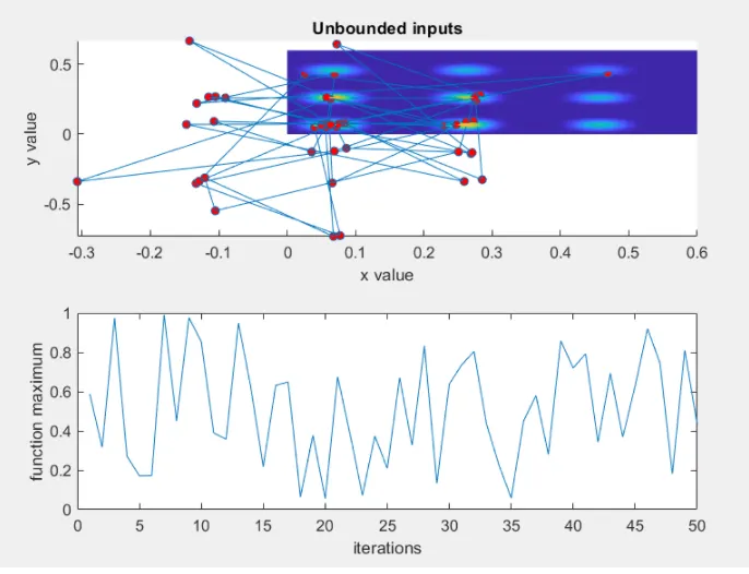
title('Unbound Inputs');
xlabel('x value');
ylabel('y value');
shading interp
hold on

plot3(xopt,yopt,-fopt,'color','b','marker','o','markersize',5,'markerfacecolor','r')
subplot(2,1,2)
plot(-fopt,'color','b','Linewidth',1)
xlabel('Iterations');
ylabel('Function Maximum');

tic;
for i = 1:num_cases
    [inputs,fopt(i)]=ga(@stalagmite,2,[],[],[],[],[0;0],[0.6;0.6]);
    xopt(i)= inputs(1);
    yopt(i)= inputs(2);
end
study_2_time = toc
figure(3)
subplot(2,1,1)
hold on
surfc(x,y,-f)
shading interp
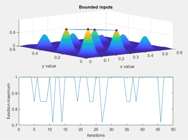
title('Bounded Inputs');
xlabel('x value');
ylabel('y value');
hold on

plot3(xopt,yopt,-fopt,'color','b','marker','o','markersize',5,'markerfacecolor','r')
subplot(2,1,2)
plot(-fopt,'color','b','Linewidth',1)
xlabel('Iterations');
ylabel('Function Maximum');

options = optimoptions(@ga)
options = optimoptions(@ga,'PopulationSize',500)

tic

for i = 1:num_cases
    [inputs,fopt(i)]=ga(@stalagmite,2,[],[],[],[],[0;0],[0.6;0.6],[],[],options);
    xopt(i)= inputs(1);
    yopt(i)= inputs(2);
end
study_3_time = toc
figure(4)
subplot(2,1,1)
hold on
surfc(x,y,-f)
shading interp
title('Bounded Inputs with Increased PopulationSize');
xlabel('x value');
ylabel('y value');
hold on

plot3(xopt,yopt,-fopt,'color','b','marker','o','markersize',5,'markerfacecolor','r')
subplot(2,1,2)
plot(-fopt,'color','b','Linewidth',1)
xlabel('Iterations');
ylabel('Function Maximum');

Output:

Explanation:

1. The 'x' ray and 'y' ray is defined using 'linspace' command to create values at 150 equal intervals.
2. A 2D mesh of x and y ray is created by using 'meshgrid' command and the number of iterations or cases that the code should perform is defined. This is given by n = 50.
3. For loop is used to evaluate the stalagmite function.
4. The input vector values of 'xx' and 'yy' are defined and the stalagmite function for these input vector is defined. This will form a basic stalagmite function and we can plot it separatelt if needed.
5. Next step is to obtain the results for 3 cases of the genetic algorithm.
6. tic and toc command is used to know the time taken. To neglect the grid lines we use shade interp.
7. The plot3 command plots the 3D points
8. After plotting result for study2, we increase the number of iterations to avoid termination of program.
9. In study3 we increase the number of iterations.

ERRORS:

No major error observed while programming.

REFERENCES:

https://in.mathworks.com/discovery/genetic-algorithm.html

https://in.mathworks.com/help/gads/how-the-genetic-algorithm-works.html