Project 1 - Parsing NASA thermodynamic data

AIM: To write a code im MATLAB to parse the NASA thermodynamic data file and to calculate the thermodynamic properties of various gas species.

OBJECTIVE:

1. To write a function that extracts the 14 co-efficients and calculates the specific heat, enthalpy and entropy for all the species in the data file.
2. To calculate the molecular weight of each species and display it in the command window.
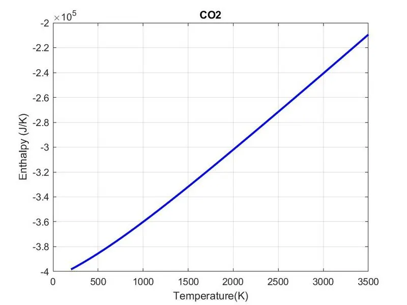
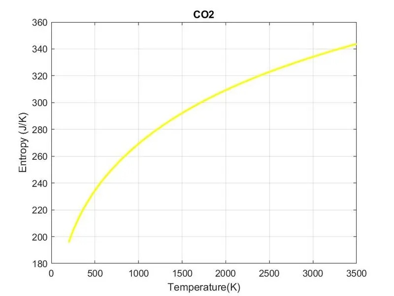
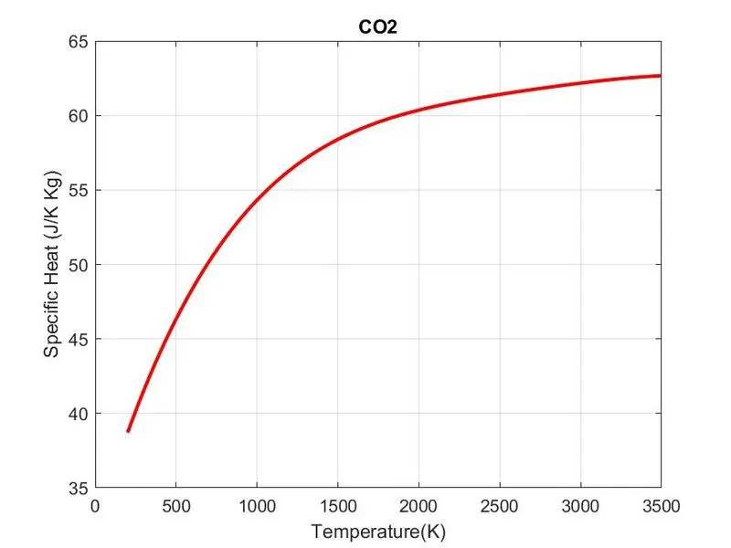
3. To plot Cp, Enthalpy and Entropy for the local temperature range (low temperature : high temperature) specific for each species.
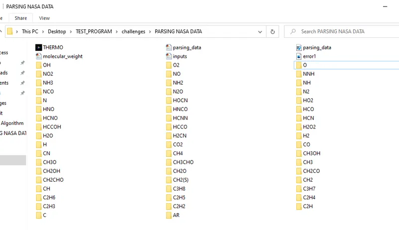
4. To Save the plots as images with appropriate names and dump them in separate folders for each species with suitable name and it should be generated automatically.

THEORY:

File parsing:

It is the method of splitting the file or other input into a piece of data that can be easily stored or manipulated. By doing this we are going to split a string into parts and then recognizing the parts to convert it into something simpler than a string.

Here in this project we are going to split the NASA thermodynamic data having 53 gas species values in 213 lines. Now, to perform the calculation for thermodynamic properties, we need some sort of co-efficients values and temperature ranges which is available in the NASA file.

Specific Heat: Specific heat is the amount of heat energy required to raise the temperature of body per unit of mass. It is also known as specific heat capacity or mass specific heat. In SI units, specific heat is the amount of heat in joules required to raise temperature of 1gm of a substance by 1 kelvin.

Enthalpy: It is a property of a thermodynamic system, is the sum of the system's internal energy and the product of its pressure and volume. It is a state function used in many measurements in chemical, biological, and physical systems at a constant pressure, which is conveniently provided by the large ambient atmosphere. In SI system, the unit of measurement for enthalpy is the joule.

Entropy: Entropy is a scientific concept as well as a measurable physical property that is most commonly associated with a state of disorder, randomness, or uncertainty.

Gas constant: The gas constant is a physical constant denoted by R and is expressed in terms of units of energy per temperature increment per mole. The gas constant value is equivalent to Boltzman constant but expressed as the pressure volume product instead of energy increment as per rise in temperature.

Molecular weight: It is the measure of the sum of the atomic weight values of the atom in a molecule.

Governing Equations:

Sample NASA data:

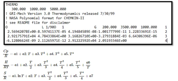
where,

Cp = Specific Heat(J/K kg)
H = Enthalpy(J)
S = Entropy(J/K)
R = Universal Gas constant = 8.314 J/mol K
T = Temperature (K)

Function Code for inputs:

In this we have developed the function for the inputs. Here the temperature varies from each species where first 7 will be local high temperature and the next 7 will be local low temperature. We have used if else command to calculate both temperatures.

CODE:

function [Cp,H,S] = inputs(T,R,Tm1,c1,c2,c3,c4,c5,c6,c7,c8,c9,c10,c11,c12,c13,c14)
for i = 1:length(T)
    if T(i)>Tm1
        Cp = (c1 + c2.*T + c3.*T.^2 + c4.*T.^3 + c5.*T.^4).*R;
        H = (c1 + (c2.*T)./2 + (c3.*T.^2)./3 + (c4.*T.^3)./4 + (c5.*T.^4)./5 + c6./T).*T.*R;
        S = (c1.*log(T) + c2.*T + (c3.*T.^2)./2 + (c4.*T.^3)./3 + (c5.*T.^4)./4 + c7).*R;
    else
         Cp = (c8 + c9.*T + c10.*T.^2 + c11.*T.^3 + c12.*T.^4).*R;
        H = (c8 + (c9.*T)./2 + (c10.*T.^2)./3 + (c11.*T.^3)./4 + (c12.*T.^4)./5 + c13./T).*R;
        S = (c8.*log(T) + c9.*T + (c10.*T.^2)./2 + (c11.*T.^3)./3 + (c12.*T.^4)./4 + c14).*R;
    end
end
end

Function Code for molecular weight:

The molecular weight is calculated using function command. Atomic weight and atomic name were given as inputs to the species. A loop is created to calculate the molecular weight of each. The string are converted to numbers by str2num command.

% Molecular weight calculation

function molecular_weight_calculation = molecular_weight(sp_name)

species = sp_name

elements = ['H','C','O','N','A','S'];
atomic_weight = [1.00794 12.0107 15.999 14.0067 39.948 32.065];

molecular_weight_calculation = 0;
 for i = 1:length(species)
     for j = 1:length(elements)
     if strcmp(species(i),elements(j))
         molecular_weight_calculation = molecular_weight_calculation + atomic_weight(j);
         a = j;
     end
 end

 n = str2num(species(i));
 if n>1
     molecular_weight_calculation = molecular_weight_calculation + atomic_weight(a)*(n-1);
 end
end

Program Code:

% Parsing NASA Thermodynamic Data
clear all 
close all
clc

f1 = fopen('THERMO.DAT','r') %opens the file for reading
fgetl(f1);   
tline = fgetl(f1);
A = strsplit(tline,' ');
Global_low_Temperature = str2num(A{2});
Global_mid_Temperature = str2num(A{3});
Global_high_Temperature = str2num(A{4});

% Eliminating the lines
for i = 3:5
    b = fgets(f1);
end


% Getting the temperature & co-efficients for each species
 for j = 1:53
     species = fgetl(f1);
     t = findstr(species,'.');

% Local temperatures for each species

species(52-3:52+3);
Tl = species(52-3:t(1)+3);
Tl1 = str2num(Tl);

species(t(1)+6:62+3);
Th = species(t(1)+6:t(2)+3);
Th1 = str2num(Th);

species(t(2)+6:72+3);
Tm = species(t(2)+6:t(3)+3);
Tm1 = str2num(Tm);
m = strsplit(species,' ')

sp_name = m{1};

% co-efficients of each species

coeff_line_1 = fgetl(f1);
A11 = strfind(coeff_line_1,'E');
coeff_line_1(1:12+3);

a1 = coeff_line_1(1:A11(1)+3);
c1 = str2num(a1);
a2 = coeff_line_1(A11(1)+4:A11(2)+3);
c2 = str2num(a2);
a3 = coeff_line_1(A11(2)+4:A11(3)+3);
c3 = str2num(a3);
a4 = coeff_line_1(A11(3)+4:A11(4)+3);
c4 = str2num(a4);
a5 = coeff_line_1(A11(4)+4:A11(5)+3);
c5 = str2num(a5);

coeff_line_2 = fgetl(f1);
A12 = strfind(coeff_line_2,'E');
coeff_line_2(1:12+3);

a6 = coeff_line_2(1:A12(1)+3);
c6 = str2num(a6);
a7 = coeff_line_2(A12(1)+4:A12(2)+3);
c7 = str2num(a7);
a8 = coeff_line_2(A12(2)+4:A12(3)+3);
c8 = str2num(a8);
a9 = coeff_line_2(A12(3)+4:A12(4)+3);
c9 = str2num(a9);
a10 = coeff_line_2(A12(4)+4:A12(5)+3);
c10 = str2num(a10);

coeff_line_3 = fgetl(f1);
A13 = strfind(coeff_line_3,'E');
coeff_line_3(1:12+3);

a11 = coeff_line_3(1:A13(1)+3);
c11 = str2num(a11);
a12 = coeff_line_3(A13(1)+4:A13(2)+3);
c12 = str2num(a12);
a13 = coeff_line_3(A13(2)+4:A13(3)+3);
c13 = str2num(a13);
a14 = coeff_line_3(A13(3)+4:A13(4)+3);
c14 = str2num(a14);
% creating the folder to save the plots
mkdir('C:\Users\Goldi Raikwar\Desktop\TEST_PROGRAM\challenges\PARSING NASA DATA',sp_name)
% Calculating the specific heat, Enthalpy & Entropy

T = linspace(Tl1,Th1,100);
R = 8.314;

[Cp,H,S] = inputs(T,R,Tm1,c1,c2,c3,c4,c5,c6,c7,c8,c9,c10,c11,c12,c13,c14);

% plotting
figure(1)
plot(T,Cp,'linewidth',2,'color','r')
grid on
title(sp_name)
xlabel('Temperature(K)')
ylabel('Specific Heat (J/K Kg)')

figure(2)
plot(T,H,'linewidth',2,'color','b')
grid on
title(sp_name)
xlabel('Temperature(K)')
ylabel('Enthalpy (J/K)')

figure(3)
plot(T,S,'linewidth',2,'color','y')
grid on
title(sp_name)
xlabel('Temperature(K)')
ylabel('Entropy (J/K)')

% changing the directory
% program = (['C:\Users\Goldi Raikwar\Desktop\TEST_PROGRAM\challenges\PARSING NASA DATA\species',sp_name]);
cd(sp_name)

% saving the plot
saveas(figure(1),'Specific Heat.jpg')
saveas(figure(2),'Enthalpy.jpg')
saveas(figure(3),'Entropy.jpg')

% cd('C:\Users\Goldi Raikwar\Desktop\TEST_PROGRAM\challenges\PARSING NASA DATA')
cd ..
molecular_weight_calculation = molecular_weight(sp_name)

end

fclose(f1)

Code Explanation:

1. The program begins with clear all, close all and clc commands to free up the command window and the workspace.
2. We will then read the data from the external NASA thermodynamic data file using fpen command which is used to open the file and fgetl command which is used to read the content in the file line by line.
3. After opening the file we will be assigned to variables called f1. Thus the fget(f1) is the command acts like a line cursor, which will retrieve the next time while running this command for the second time and so on.
4. Now, we will be skipping the first 5 lines by using for loop to enter the pattern of values of the respective gas species. we will be using the for loop command to process the same for all the gas species.
5. The name of the gas species we will be found out using findstr command and for finding out the species we are going to locate the string which is present in after each species name.
6. The local temperatures for the respective gas species if found similarly using findstr command and we are going to locate the string using which we will find out the values of the low, mid and high temperature which is assigned to the variables Tl,Tm and Th respectively. But the values we have coefficients are string values so we have to change these string values to numeric values using str2num command.
7. Now, we are going to extract the coefficients for the gas species in which the co-efficient locations are like in the 2rd row, followed by next 5 in the 3rd row and the rest in the 4th row.
8. We are going to extract this value similarly we did for finding out the local temperatures by using the findstr and str2num commands and store it in the variables a1 to a14. For extracting we are going to locate the string 'E' which is present in each coefficient value and so it will be followed for all teh co-efficients values in the same line and then we can proceed for the next lines.
9. The values from a1 to a7 represents the high temperature coefficients and the values from a8 to a14 represents the low temperature.
10. Temperature range values from low temperature to high temperature is assigned using the linspace command.
11. The for loop command is used to calculate the values of specific heat, enthalpy and entropy and the if-else command is used to find the required values if the temperature is below the mid temperature or above the mid temperature.
12. Now, for loop command is used to detect if there are more than one species in the variable sp_name and the respective values of the gas species values are calculated and found out.
13. After the nested for loop the sp_name which is in the form of string is converted as number with strdouble command. Then the sp_name which is now as number is greater than one. Molecular weight is again calculated by having the atomic mass for the current species * n-1.
14. The values of molecular weight is calculated for the respective gas species and displayed in the command window.
15. Now, we are going to create plot for the obtained specific heat, enthalpy, entropy values and save it in repective folder name automatically.
16. mkdir command is used to create new folder in the main folder. Then we have to change the directory from the main folder to the folder named species_name and to perform this we use cd command.
17. The plot for specific heat vs temperature, enthalpy vs temperature and entropy vs temperature is plotted. The labeling of axis and naming of the title is also done along with the value of molecular weight.
18. To save the plot in the sp_name folder, saveas command is used. Then we change the current directory to the main folder by oldfolder = cd.. .

RESULTS:

Screenshot of the saved files:

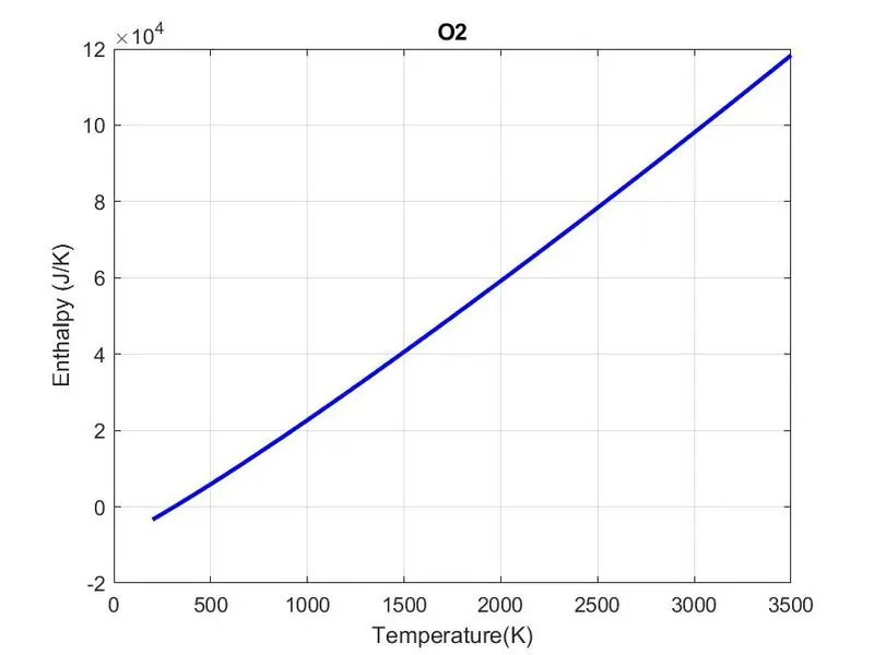
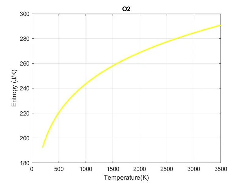
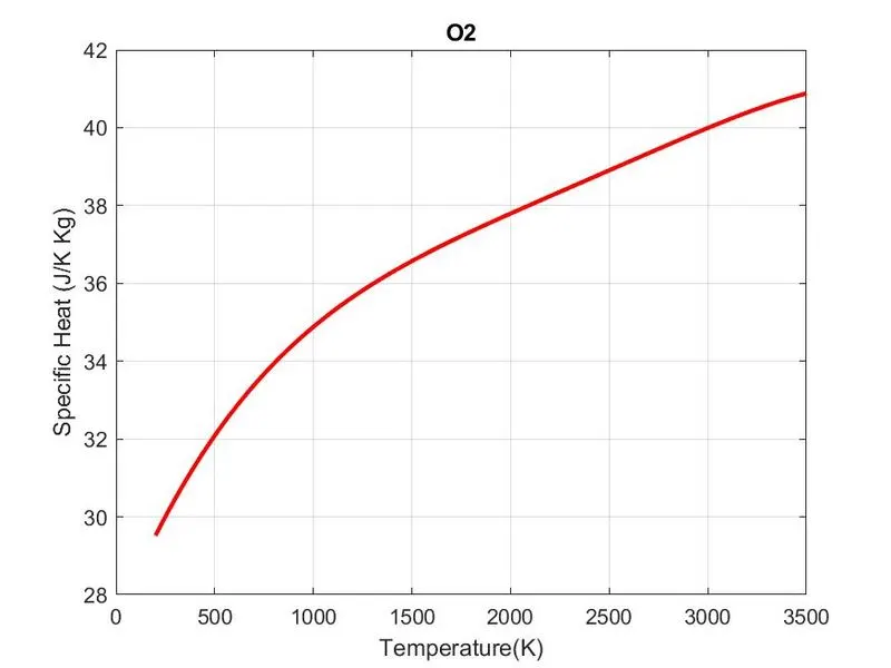
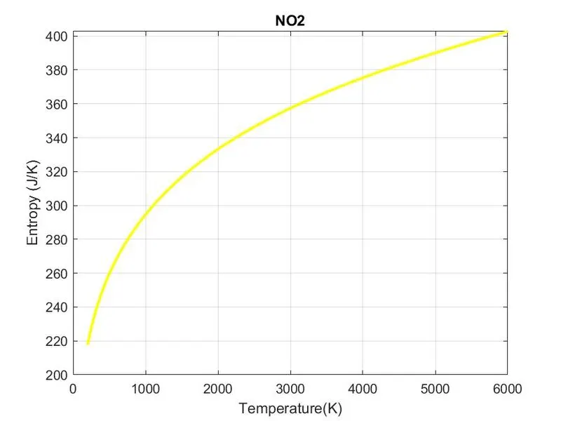
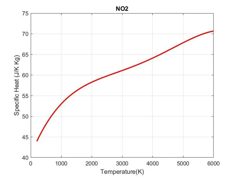
Plots for O2,NO2 and CO2 species:

a. Plots for O2:

b. Plots for NO2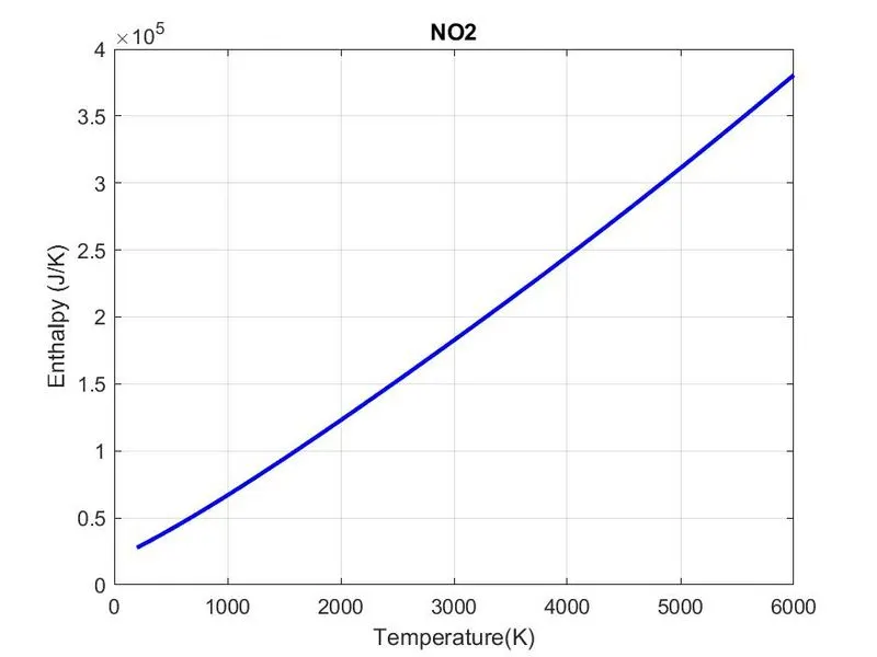

c.Plots for CO2

CONCLUSION:

Therefore, we have successfully parsed the given NASA thermodynamic data file and plotted the graphs of specific heat, enthalpy and entropy for the given inputs.

Parsing is very important part of many computer science disciplines. It is helpful to extract and read the data's from different sources.

References:

https://en.wikipedia.org/wiki/Parsing

https://en.wikipedia.org/wiki/Entropy

Matlab help

Support engineers help