Week 3 - Solving second order ODEs
INTRODUCTION:
A simple pendulum can be described as a device where its point mass is attached to a light inextensible string and suspended from a fixed support. The vertical line passing through the fixed support is the mean position of a simple pendulum. The vertical distance between the point of suspension and the centre of mass of the suspended body (when it is in mean position) is called the length of the simple pendulum denoted by L. This form of the pendulum is based on the resonant system having a single resonant frequency.
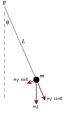
A simple pendulum consists of a mass m hanging from a string of length L and fixed at a pivot point P. When displaced to an initial angle and released, the pendulum will swing back and forth with periodic motion. By applying Newton's second law for rotational systems, the equation of motion for the pendulum may be obtained
 ,
,and rearranged as

 .
.The simple harmonic solution is

In Engineering, ODE is used to describe the transient behavior of a system. A simple example is a pendulum.The way the pendulum moves depends on the Newtons second law. When this law is written down, we get a second order Ordinary Differential Equation that describes the position of the "ball" w.r.t time
AIM: To solve the second order ODE using MATLAB which depicts the motion of the simple pendulum and to create an animation of the same.
OBJECTIVE: To write a program to solve second order ODE. The ODE represents the equation of motion with damping coefficient.
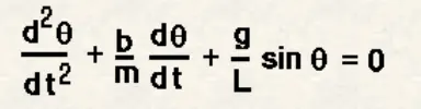
where,
g = acceleration due to gravity in m/sec^2
L = Length of the pendulum in m
b = damping coefficient
m = mass of ball in kg
Given Parameters
L=1 metre,
m=1 kg,
b=0.05.
g=9.81 m/s2.
Time period = 0-20 sec.
Angular displacement=0
Angular velocity=3 rad/sec at time t=0.
Function Code:
function [dtheta_dt] = ode_function(t,theta,b,g,l,m)

theta1 = theta(1)
theta2 = theta(2)
dtheta1_dt = theta2;
dtheta2_dt = -(b/m)*theta2 - (g/l)*sin(theta1);
dtheta_dt = [dtheta1_dt ; dtheta2_dt];

end
Explanation:
1. In this function program the second order ODE is simplified to first order ODE by introducing the term theta1 and theta2
2. Then theta1 and theta2 are differentiated to get dthet_dt matrix.
Program Code:
clear all
close all
clc

% Damping coefficient
b = 0.05;
% Acceleration due to gravity(m/s^2)
g = 9.81;
% Length (m)
l = 1;
% Mass (Kg)
m = 1;

% initial condition
theta_0 = [0;4];

% time points
t_span = linspace(0,20,200);

% solving ODE
[t, results] = ode45(@(t, theta) ode_func(t, theta, b,g,l,m),t_span,theta_0);

% Animation
ct = 1;
for i = 1:length(results(:,1))
    x0 = 0;
    y0 = 0;
    x1 = l*sin(results(i,1));
    y1 = -l*cos(results(i,1));

    plot([x0 x1],[y0 y1],'-o','Markersize',10,'Markerfacecolor','r','MarkerEdgecolor','r','linewidth', 5)
    axis([-1.5 1.5 -1.5 1.5])
    hold on
    plot([-1 1],[0 0],'linewidth',5, 'color', 'b')
    hold off
    M(ct) = getframe(gcf);
    ct = ct + 1;
end

% Movie and Videofile
movie(M)
videofile = VideoWriter('ode_main.avi','Uncompressed AVI')
open(videofile)
writeVideo(videofile,M)
close(videofile)

% plotting
plot(t, results(:,1))
hold on
plot(t,results(:,2))
xlabel('Time')
ylabel('Velocity(Red) & Dispalcement(Blue)')
Explanation:
1. In this program first we mentioned the provided fixed parameters which are length, mass, damping coefficient and acceleration due to gravity.
2. Time and angle is given as initial condition.
3. In the tspan command 200 values are taken for 0 to 20 time period.
4. using the ode45 command, ODE fucntion is introduced.
5. Then we plotted the velocity, displacement vs time graph.
6. By using for loop command the mass at various points and various time is plotted.
7. Using the movie command the video file is saves as uncompressed AVI file.
PLOTS:
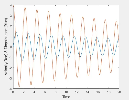
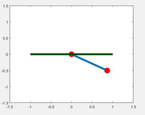
Screenshots:
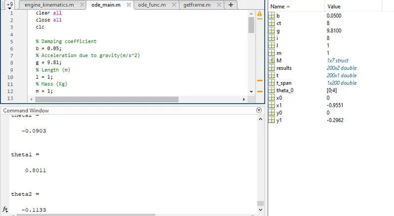
Animation:
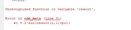
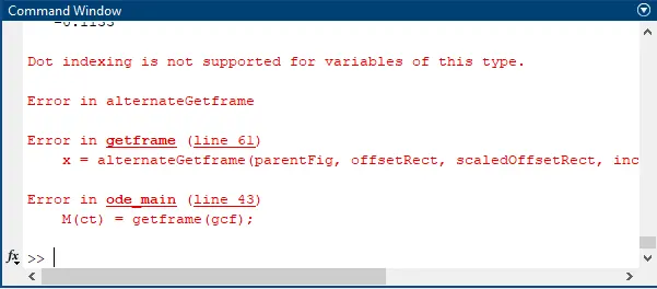
Errors:
A typo error that got corrected by inspecting.


Got corrected by removing the figures and evaluate.
Youtube link for the animation:
https://youtu.be/6MZnXoKtqUs